Polluting the Internet

AGU 2013 Days 4 & 5: measurements & models

Will Morgan December 14, 2013

My fourth and fifth days at the AGU Fall Meeting involved dashing between multiple sessions to take in a number of talks on (surprise, surprise) aerosols! The main strand running through them from my point of view was how there are major efforts to construct large datasets of aerosol properties that can be used to test our understanding via numerical models.

Aerosols are complex and tend to stick around in the atmosphere for hours-to-weeks, rather than years-to-centuries. This means that they are spatially very diverse and also vary with time e.g. with the passage of seasons. This presents a challenge for our understanding but by constructing large datasets, it can also be used to constrain our numerical models.

For example, by looking at years of winter data for European pollution we might find that our models represent this quite well but it might be that there are significant errors when we look at the summer. This information is useful and might point us towards places to study further and improve our understanding. Just looking at a global annual average, this information is lost.

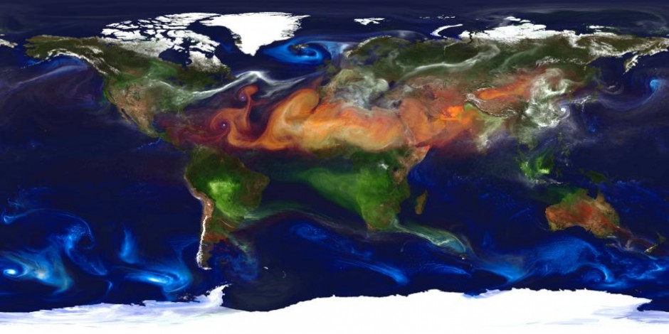
Image of the global aerosol distribution produced by NASA. The image was produced using high-resolution modelling by William Putman from NASA/Goddard. The colours show the swirls of aerosol particles formed from the numerous sources across the globe. The colours show aerosol particles as dust (gold/brown), sea-spray (blue), biomass burning/wildfires (green) and industrial/urban (white).

There were several talks detailing efforts to build satellite data sets of aerosol properties over long periods and use these to assess numerical models. Phillip Stier from the University of Oxford sounded a cautionary note by illustrating how different satellites can sometimes deliver different results for certain properties. He showed three different satellite images of cloud effective radius, which is a property of clouds that is important for how they interact with sunlight, and they were all very different. One of them agreed with his model but which set of measurements do you believe? He ended with a call to expand initiatives that seek to collate data from surface and aircraft measurements to test satellite measurements and models.

Dan Murphy from the National Oceanic & Atmospheric Administration paper presented some work on trends in aerosol over the past decade. He showed that while at a global level, the amount of aerosol in the atmosphere hasn’t really changed, it has changed significantly at the regional level. Aerosol concentrations have decreased in the USA and Western Europe, while they have increased in East Asia and in the Middle East. Aerosol has moved around a lot but there has not been a discernible change in their radiative effect at the global level. However, he said we couldn’t rule out that aerosols haven’t caused other adjustments such as circulation changes and clouds. You can access his Nature Geoscience paper on his work here. His work is consistent with several other papers that have shown negligible trends in global aerosol after the past decade.

These were highly interesting talks and should serve us well as we attempt to improve our understanding of aerosols, although there is much work still to do. No doubt we can anticipate much more work on this in the future – one of the talks did proclaim that:

Aerosol reanalysis is trendy.

No doubt we’ll be seeing the influence of this in the fashion houses of London, Paris and New York soon.

AGU 2013 Day 3: secondary organic aerosol – animal or vegetable?

Will Morgan December 12, 2013

My third day at the AGU 2013 Fall Meeting involved lots of talks on one of the trickiest parts of aerosol science – secondary organic aerosol (SOA). We’ve known for several years now that SOA is ubiquitous across the globe and it is often the most dominant aerosol chemical species in many environments and this is particularly true in the industrialised regions of the Northern Hemisphere. The trouble, we’re not sure where it comes from and how it forms…

SOA represents the carbon-containing fraction of atmospheric aerosol that forms as a consequence of chemical processes in the atmosphere. Instead of being directly emitted in particle form e.g. from a car exhaust, they form from gases known as volatile organic compounds (VOCs) which can be emitted by both ourselves via burning fossil fuels or from natural sources such as trees. This latter glass of “biogenic” compounds is what gives pine trees and others their distinctive smell.

Morning fog in the Great Smoky Mountains. Image from EGU Imaggeo image repository and is provided by Oliver Pratt.

Morning fog in the Great Smoky Mountains. See also the haze in the background in the top left. Image from EGU Imaggeo image repository and is provided by Oliver Prat.

An area where there are large emissions of these biogenic compounds is the South-East of the USA and they are responsible for the ‘smokiness’ of the Great Smoky Mountains, which are pictured above. The SE USA is also interesting as parts of it have not warmed like other parts of the USA due to global warming – in fact, some areas have actually shown a cooling trend. One theory is that aerosols formed from the biogenic compounds are involved.

Many of the talks on SOA this week have been based on measurements from an array of projects that took place in the SE USA in 2013. Some of the main themes/conclusions include:

SOA from biogenic emissions of a VOC called isoprene are an important component. Isoprene is the most abundant biogenic VOC worldwide (aside from methane), so it potentially represents a large source of SOA.
Several of the measurements showed a strong link between isoprene SOA and sulphate aerosol, which is typically from human sources such as power plants. This is consistent with the work of Jason Surratt’s group and others. This is particularly important as it demonstrates how emissions from human activities can interact with biogenic emissions to form pollution, which was postulated to be important by Allen Goldstein in 2009. Yet another example of our impact on the atmosphere.
Condensed water is a significant part of aerosols in the SE USA, which is important for the impact of aerosol on climate. However, the evidence for it being a major driver of SOA formation, as suggested by Annmarie Carlton was limited. Further studies are required klaxon!
ISOPOOH is an important oxidation product of isoprene that forms when Tigger and Winnie have an argument and potentially leads to SOA formation.

New toys

Overall, the talks on SOA from these measurement studies were a fantastic demonstration of many of the new techniques to characterise SOA. These new techniques will certainly improve our understanding of SOA formation, particularly in areas where large volumes of our own emissions interact with the biogenic emissions.

AGU 2013 day 2: aerosol emissions, climate & the IPCC

Will Morgan December 11, 2013

My second day at the AGU 2013 Fall Meeting revolved around more short-lived climate forcers, which I wrote about yesterday and also a broader session on the results from the recent IPCC Working Group 1 report. The latter was an opportunity for the community to quiz some of the lead authors of the report on a variety of issues including observations of the climate system, aerosol and clouds (yippee!), carbon cycle feedbacks, sea level rise and future changes.

Oliver Boucher gave a very nice overview of the aerosol and clouds chapter that he was a coordinating lead author for. I suspect it was a condensed version of the presentation he gave at the “Next steps in climate science“ meeting at the Royal Society, which I summarised here previously.

Desert fires feeding a convective cloud system over Mono Lake, California. Image from EGU Imaggeo image repository and is provided by Gabriele Stiller.

Smoke aerosol feeding a convective cloud system over Mono Lake, California. Image from EGU Imaggeo image repository and is provided by Gabriele Stiller.

One of the key messages for me was his conclusion that there has been substantial improvements in our understanding of aerosol and cloud processes since the previous IPCC report in 2007 but that this ‘knowledge’ hasn’t quite made its way into current global climate models. As someone who works on understanding aerosol processes from observations of the ambient atmosphere, this is something I very much agree with! The implication here is that aerosol uncertainty will reduce in the future as this knowledge is translated to future climate models. We can but hope.

Some of the other key points from his talk included:

Confidence in satellite based global average aerosol optical depth trends is low.
Black carbon dominates uncertainty in aerosol radiative forcing.
Many gaps in understanding including absorption by black carbon, trends and circulation changes due to aerosol forcing.
Low level clouds are the “joker in the pack” of cloud feedbacks as they are the least understood area for clouds.

Still plenty of work to do!

Emission reductions

The short-lived climate forcers session in the afternoon included a very nice study of how emission regulations in California have affected air pollutant emissions, including black carbon. Tom Kirchstetter presented measurements of trucks using the Oakland port just across the bay from the AGU venue in San Francisco. The neat thing about the study was that this was done over several years both before the regulations were in place and afterwards. The regulations required diesel particle filters to be installed in new trucks, while old trucks had to be retro-fitted with them.

These new regulations have seen an 80% decrease in black carbon emissions over 4 years. The reduction is about 5-times faster than ‘natural’ fleet turnover, which occurs more gradually as new vehicles with improved engines replace older models. The new rules apply to 10,000-20,000 vehicles and will likely significantly improve air quality in the area. Further regulation will soon come into force for 1 million buses and trucks, which could have profound impacts on black carbon emissions in California.

This will likely be an interesting area to keep an eye on in terms of the wider potential impacts on air quality and climate.

AGU 2013 day 1: Short-lived climate forcers

Will Morgan December 10, 2013

My first day at AGU 2013 revolved around sessions on short-live climate forcers, which are components in the atmosphere that have short lifetimes (compared to carbon dioxide for example) and generally warm the atmosphere. Reduction of these compounds, such as methane and black carbon, has been mooted as a way to reduce global mean temperatures in coming decades.

This is summarised in the figure below, where the modelled impact of reducing black carbon and methane alongside reductions in carbon dioxide emissions are shown. The majority of the benefit in reducing methane and black carbon is felt by 2040 – if you look at longer time scales, then the effect diminishes relative to carbon dioxide.

Modelled impact of various reductions in carbon dioxide, methane and black carbon (BC) on global mean temperature. Figure courtesy of UNEP Integrated Assessment of Black Carbon and Tropospheric Ozone.

The problem with this idea is that there is much uncertainty related to these short-lived components, so it isn’t clear how much global temperatures would respond to a reduction in their atmospheric concentrations. This is represented in the above figure by the vertical bars to the left of the graph – there is much overlap here, which reflects this uncertainty. The health benefits of reducing black carbon in particular are quite clear though. Most of the talks focussed on black carbon and that is what I am also going to focus on below.

Fuzzy metrics

Tami Bond made some excellent and thought-provoking points on how short-lived climate forcers are framed relative to carbon dioxide. The key property for black carbon in the framework of near-term reductions in global temperature is its short lifetime in the atmosphere (days-to-weeks). This means that it is not evenly distributed across the globe, unlike greenhouse gases such as carbon dioxide and methane. This results in its radiative forcing being spatially distinct – the perturbation it has on our planets energy balance occurs close to its source of emission. The impact of such changes is usually felt more at the regional level, rather than the global scale associated with carbon dioxide. Her main point was that this is then an apples-to-oranges comparison, so for example, reducing black carbon emissions in Asia might not have a great impact of global mean surface temperatures but it may well reduce temperatures in the region and slow the effects of carbon dioxide driven warming.

She also reiterated the difficulties associated with the pollutants that are co-emitted with black carbon, which complicate the picture and are one of the major reasons that there is substantial uncertainty surrounding reducing black carbon. In the real world, you can’t really just reduce black carbon – any technological solution will likely perturb the other pollutants, which tend to cool our climate. Attempts to reduce black carbon might actually result in temperatures rising – I’ve written more on studies that have considered this here.

Other highlights

Yi Deng presented a fascinating study of how aerosol particles can influence the atmosphere far away from their actual location by modelling the impact of biomass burning in Southern Africa on the Asian Summer Monsoon. He showed that the substantial burning that occurs actually strengthens the monsoon by inducing circulation changes up-wind of the Indian sub-continent and south-east Asia. We tend to think of aerosol impacts being confined to their atmospheric location but this illustrated how joined-up our atmosphere is.

One of the issues with black carbon is that some sources have received little attention previously. Ed Fortner from Aerodyne Research Inc. presented measurements of emissions from brick kilns in Mexico, which produce a lot of black carbon. There are around 300,000 kilns worldwide producing 1.5 billion bricks per year! Over half of these are in China (54%), with India (11%), Pakistan (8%) and Mexico (7%) being the other major kiln hotspots. Characterising the emissions from these and other sources is likely going to be in important for efforts to constrain the impact of black carbon on both our climate and health.

Chris Cappa presented follow-up work to his 2012 paper in Science that investigated how much warming by black carbon is enhanced by other aerosol species that coat it. Black carbon warms the atmosphere by absorbing sunlight and both laboratory and theoretical evidence suggests that this is increased by coatings on the black carbon particles. This coating focusses sunlight onto the black carbon core, like a magnifying glass held to the sun does and this increases the absorption by the black carbon, a phenomenon known as “lensing”. Chris has been busy testing how much enhancement we see in the real world using measurements and typically to enhancement ranges from 10-30%, which is lower than is often suggested by aerosol models. There are significant caveats here as the measurements are challenging and require the aerosols to be “dry” – this is important as water often condenses onto aerosol particles and increases their reflective and lensing ability. This could be a vital ingredient in this process and it is a significant challenge to overcome.

My final highlight was presenting my poster! The AGU poster hall is absolutely massive and must span several football pitches. Despite this, the sessions are hugely rewarding and are a great opportunity to discuss science with a variety of people. The posters are a major part of the AGU fall meeting, which is not always true of other conferences. I’m looking forward to roaming the hall now that my own poster is done.

Me presenting my poster on day 1 of AGU 2013. Image courtesy of Sam Illingworth.

Communicating uncertainty

With all this complexity revolving around black carbon and the interest it has received from policy makers, Tami Bond was asked how to communicate this to non-scientists. Her response was:

Keep it simple but don’t ignore physical reality.

That seems like a pretty good mantra to me.