Biomass burning

Around the world

Will Morgan January 14, 2015

The short lifetime of aerosol particles in the atmosphere means that they tend to be found concentrated in regions close to where they were formed. As they only last for days to weeks in the atmosphere, they don’t travel too far as the Earth’s winds aren’t able to fully mix the air over such a short period.

This short lifetime should also mean that any changes in the emissions of aerosol particles and their gas-phase building blocks will show up quickly when we measure their concentrations in the atmosphere. This contrasts with greenhouse gases, which typically have much-longer lifetimes (decades to centuries), so their concentrations remain much further into the future (even if their emissions were ceased completely).

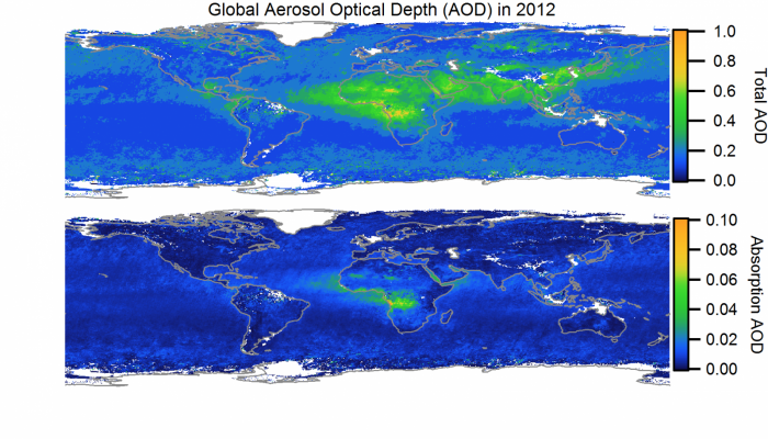
Below is a collection of images of the global aerosol view from 2001 to 2012 from the Multi-angle Imaging SpectroRadiometer (MISR) on board NASA’s TERRA satellite. Each map is a single year, with the year noted to the bottom right of the image. The maps show the Aerosol Optical Depth (AOD), which is a measure of the amount of aerosol within the atmosphere. As the measurements are made from space, the instrument measures the aerosol in a vertical column below the satellite. Terra orbits the Earth continuously and gradually builds up a picture of the Earth below; MISR itself will typically build up a global picture over a couple of weeks.

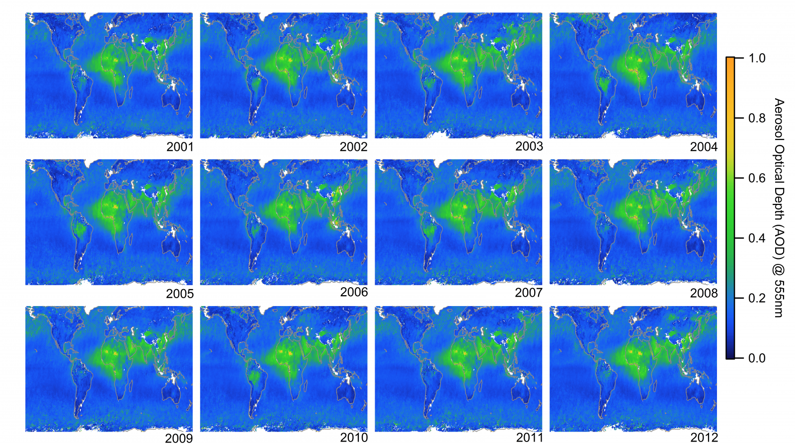
Global view of the Aerosol Optical Depth (AOD) from 2001-2012 observed by the Multi-angle Imaging SpectroRadiometer (MISR) on board NASA’s TERRA satellite. White spaces indicate there is no data. High latitudes are excluded as the satellite retrievals don’t work over highly-reflective surfaces (snow/ice). Click on the image for a larger view.

The most persistent feature is the large expanse of aerosol over Africa, which also extends into the Atlantic Ocean. Over North Africa, much of this aerosol is a result of the wind whipping up a storm of Saharan dust, which can then be blown over large distances. Sometimes, the dust even makes its way across the whole Atlantic Ocean and lands in North or South America. Further south, frequent burning occurs to clear savannah areas in Southern Africa, which creates large amounts of smoke.

The Arabian Peninsula, India and South-East Asia (particularly China) are other regions where aerosol is prevalent. Similarly to the Sahara, Saudi Arabia is prone to large dust storms, while India and China have undergone significant economic development recently, which has led to increased burning of fossil fuels. South America also sees a large build up of aerosol over the Amazon Rainforest due to deforestation fires, although the amount of aerosol varies more from year-to-year.

Europe, North America and Australia display relatively low levels of aerosol compared to these other regions. Bear in mind that these are annual averages, so they will miss intense and short-lived pollution events, which do still affect these regions.

The atmosphere above the Earth’s oceans is generally quite clean as far as aerosol is concerned, as the major sources of aerosol are far away. There are deviations from this general observation though, for example, aerosol is transported across the Pacific Ocean from Asia to North America. This can be seen in the top right of each image (as well as in the top left at times). The strong winds in the Southern Ocean also see elevated aerosol amounts, as the wind helps to produce sea spray aerosol.

Below is a map showing the difference between the last four years shown above (2009-2012) and the first four years (2001-2004) in order to highlight changes in aerosol over this period. Overall, there hasn’t been a great change in the global amount of aerosol; Dan Murphy, in a paper in Nature Geoscience (pay walled, sorry), showed that the level of aerosol hasn’t changed much over this period but that there have been regional changes. This is in agreement with several other papers using similar and/or the same measurements (some non-pay walled papers here and here). From a statistical point of view, the trend in global aerosol is negligible and weakly positive i.e. aerosol levels have increased since the turn of the century but the increase isn’t statistically significant.

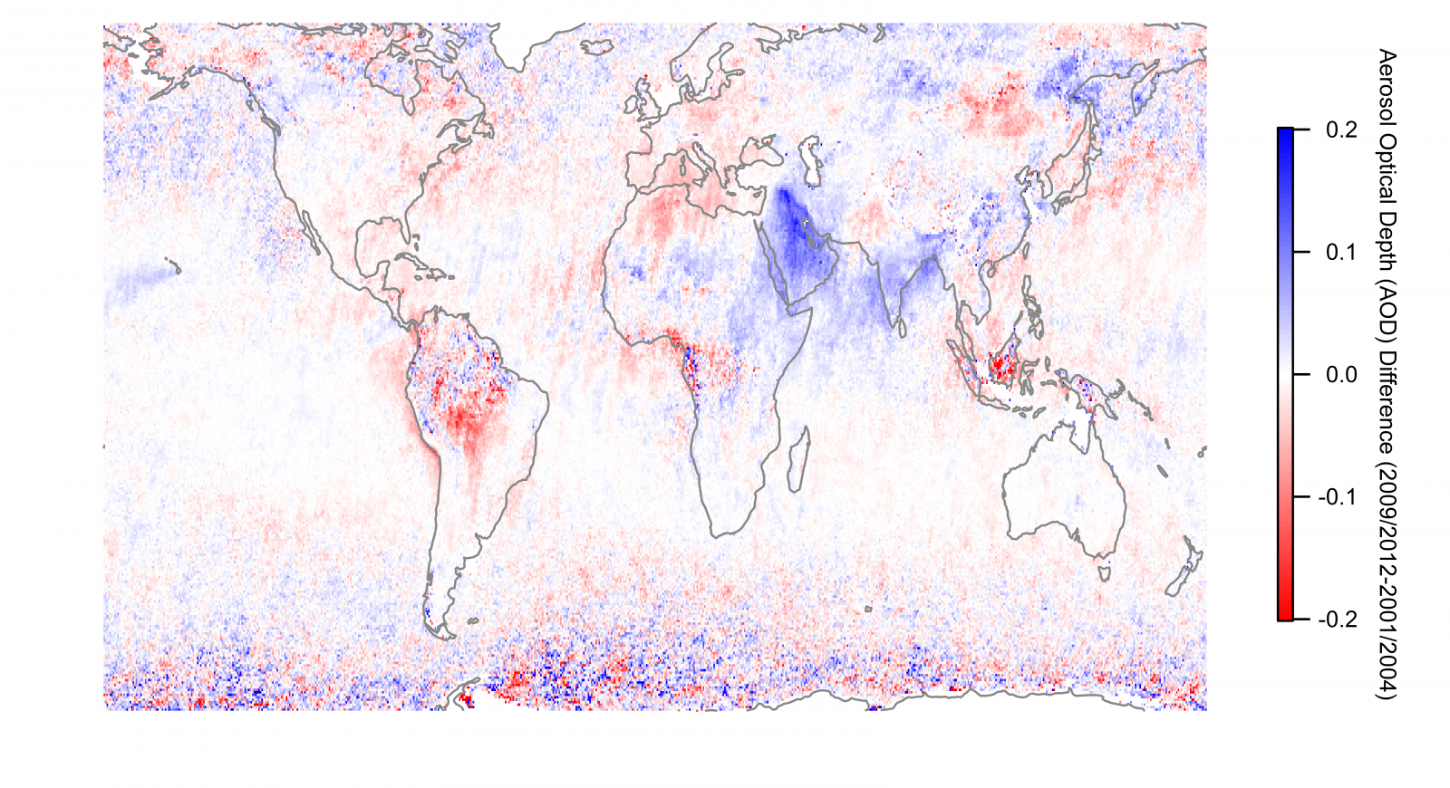
Difference in Aerosol Optical Depth (AOD) from 2009-2012 to 2001-2004. Data source is the same as above. Blue colours indicate an increase in aerosol, while red colours show a decrease.

The strongest increases have been over the Arabian Peninsula and India. These increases are likely a consequence of natural causes in the case of Saudi Arabia via increased dust emissions and transport, whereas India is likely a consequence of increased burning of fossil fuels. South America is probably the most notable region as far as aerosol decline is concerned; in recent years, deforestation has decreased compared to the early 2000s combined with some wetter years over the Amazon. Significant burning does still occur though, with 2010 being a notable year where drought conditions meant that a very large amount of smoke built up over the Amazon during the biomass burning season. There have also been declines in aerosol over Europe and the North Eastern USA, which are likely due to decreased emissions of sulphur dioxide from coal power stations.

The upshot of these trends is that since the year 2000, aerosol particles have undergone relatively minor changes on the global scale. The question going forward is whether this will continue and what impact will such changes have on our climate. Thus far, the declines in Europe and North America have been offset by increases in Asia, although the climate-relevant properties of the aerosol may not be the same. Furthermore, much of the decline in aerosol has been driven by reductions in sulphate aerosol but other species, such as secondary organic aerosol and ammonium nitrate, may become comparatively more important. These species are often missing or poorly represented in climate models, which has been suggested as an explanation for the recent pause/hiatus/slowdown in global mean surface temperature.

This is clearly a major issue in climate science currently and the role of aerosol is unclear. I’ll be writing more on this topic in the future, so watch this space!

—————————————————————————————————————————————————————–

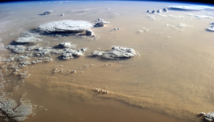
Header image: Dust and Clouds Dance Over the Sahara, published by NASA Earth Observatory. The photograph was taken by astronaut Alex Gerst on September 8, 2014, from the International Space Station.

MISR analyses and visualizations used in this blog post were produced with the Giovanni online data system, developed and maintained by the NASA GES DISC.

Wuthering heights

Will Morgan January 7, 2015

Aerosol particles typically have short life spans in the atmosphere (days to weeks) but they can travel far and wide in that time. They can be lifted up to new horizons, higher and higher in the atmosphere.

This is important for their impact on our climate, for example, at least 20% of the uncertainty in the climate impact of black carbon aerosol is due to differences in its vertical distribution. This is due to black carbon having a stronger climate impact when located higher in the atmosphere compared with black carbon at the surface.

The majority of the sources of aerosol particles are located on the Earth’s surface but through atmospheric mixing, the particles can be transported to higher altitudes. This variation in aerosol concentrations with altitude is referred to as their vertical profile.

As someone whose research has focussed a lot on aircraft measurements, aerosol vertical profiles are something I think about frequently. Below is an example of a vertical profile from a paper I wrote in 2009, which collated aerosol chemical composition data from 41 research flights around the UK over an eighteen month period.

The profile is for sulphate aerosol, which can arise from both natural sources as well as through fossil fuel burning (particularly coal burning in power plants). We can see that sulphate aerosol peaks in the lowest 3km of the atmosphere and that it varies a lot, with reduced and more consistent concentrations found in the free troposphere above 4km. At the very top of the profile, sulphate appears to increase a little, which is likely due to long-range transport of pollution.

Vertical profile of sulphate aerosol based on aircraft measurements around the UK from Morgan et al., 2009, Atmospheric Chemistry & Physics. Black and grey crosses correspond to individual data points, while the red lines in the left hand panel show the 25th, 50th and 75th percentiles for 500m altitude bins. In the right hand panel, the mean profile is shown, along with a representation of the variability in each altitude bin.

It turns out that when comparing observations of aerosol concentrations similar to those above, climate models generally have a tough time replicating the measurements. Personally, I see aerosol vertical profiles as an acid test of model performance as they are a useful means of testing various processes within the models; crucially, the shape of the vertical profile is largely independent of the emission strength of the aerosol sources (which are often highly uncertain), so any discrepancies are easier to ascribe to the processes within the model itself. Essentially, the aerosol vertical profile helps with the detective work that goes into diagnosing issues relating to our understanding of aerosol particles.

Below is an example from Hodnebrog et al. where they compared measurements of black carbon aerosol with a number of climate models. The grey shaded region shows the range from a collection of models and it is quite wide throughout the profile when looking at the 30N-60N and 30S-0 panels (A and B), with some models 10-100 times greater than others in terms of black carbon concentration. This means that there is a large diversity in what the different models think the black carbon concentration is at a given altitude. This is also true at higher altitudes over Japan; the narrower range closer to the surface is likely because the source of black carbon in this region will be from Japan itself, so the lowest portion of the profile will be strongly linked to the emissions from the surface.

Comparison between aircraft observations (black line), the AeroCom phase II model range (shaded area), the AeroCom phase II OsloCTM2 model result (dashed orange line) and various simulations with the OsloCTM2 model (coloured lines). The observations are from the HIPPO3 (a,b) and A-FORCE16 (c) campaigns. Figure is from Hodnebrog et al., 2014, Nature Climate Communications.

Now, when comparing the thick black line with the grey shaded region, we see that the observations are close to the centre of the model range over Japan (although the observations don’t extend very far in altitude). However, in the other panels, the observations are biased to the lower end of the model range and even falls outside it at high altitudes in panel A. This is a somewhat curious result, as our current understanding of black carbon is that its emissions are generally underestimated; if all else were equal, increasing the emissions of black carbon in models to reflect our current understanding would make such a comparison worse.

This over-prediction of black carbon concentrations, combined with the poor representation of the vertical profile suggests that other facets are playing a role in determining the black carbon vertical profile. The coloured lines in the figure are results from a single model using different assumptions about black carbon. The upshot of this from the paper is that the lifetime of black carbon is likely overestimated in the model, with the paper concluding that:

Increased emissions, together with increased wet removal that reduces the lifetime, yields modelled black carbon vertical profiles that are in strongly improved agreement with recent aircraft observations.

This is consistent with several other studies that have implicated the lifetime of black carbon as being responsible for the overestimation of black carbon at high altitudes. By increasing the amount of black carbon removed by precipitation, these studies can better represent the vertical profile of black carbon. The lifetime of black carbon isn’t likely to be the only culprit though and the discrepancies will likely vary geographically; in the tropics, the Coupled Model Intercomparison Project Phase 5 (CMIP5) models potentially suffer from overenthusiastic convective transport, which leads to more black carbon at higher altitudes when comparing with measurements. As ever, aerosol presents a complex picture.

Black carbon isn’t the only aerosol species subject to these issues, for example, organic aerosol also shows similarly large diversity between models and the agreement with observations isn’t particularly good.

Improving the representation of aerosol vertical profiles is a significant challenge due to a number of factors. Chief among these is the relatively sparse nature of detailed measurements of the aerosol vertical profile; airborne studies are expensive and are typically conducted for short periods e.g. month-long intensive projects. However, the number of airborne research platforms and projects is increasing rapidly, so the potential for improvements in our understanding is likely to increase as more measurements are collected and more measurement-model comparisons are conducted.

Hopefully, the answers are out in the winding, windy atmosphere.

—————————————————————————————————————————————————————–

Header image: Facility for Airborne Atmospheric Measurements (FAAM) BAe-146 research aircraft. Image courtesy of FAAM website.

Some of my colleagues are collating a vast number of measurements, with particular focus on airborne observations, for the Global Aerosol Synthesis and Science Project (GASSP), with the aim of creating a database that will be ideal for measurement-model comparisons. If you are interested, I can put you in touch with the relevant people.

If you want to hear and see more about the vertical profile of black carbon (and who doesn’t), then my presentation at AGU Fall Meeting is available online here. The registration is free and I’m told it will be available FOREVER.

The dark side of the atmosphere: the blog awakens

Will Morgan December 3, 2014

Global view of the amount of aerosol in 2012 observed by the Multi-angle Imaging SpectroRadiometer (MISR) on board NASA's TERRA satellite. The top map shows the Total Aerosol Optical Depth AOD, while the bottom map shows just the absorbing component of atmospheric aerosol. White spaces indicate there is no data. Note the different scales for each panel.

Aerosol particles come in lots of different flavours and one of their most important properties is how they deal with incoming sunlight. Some are rather unwelcoming and send sunlight back to whence it came (space), which leads to a cooling of the atmosphere as the sunlight doesn’t reach the surface of the Earth. Others offer sunlight a warm(ing) embrace and absorb it, which heats up the atmosphere.

The relative amount of absorbing aerosol compared to the total aerosol burden in the atmosphere is the primary control on whether aerosol particles have a warming or cooling impact. Overall, aerosol particles are thought to cool climate but there are differences regionally and over the course of a typical year. We can see in the maps above that the absorbing aerosol is typically much smaller than the total amount of aerosol; the absorbing fraction is generally less than 5% of the total.

Regionally, the level of absorption and its relative contribution can be much larger, particularly where large-scale biomass burning occurs. Southern-West Africa sticks out in the above image where large-scale biomass burning occurs frequently. These open fires release large amounts of black carbon, which is the major absorbing aerosol species in the atmosphere. In addition, the fires can release so-called ‘brown carbon‘, which is a more weakly absorbing aerosol made up of organic material.

To complicate matters, biomass burning aerosol is also made up of the unaccommodating aerosols that scatter sunlight back to space. The competition between the scattering and absorbing aerosol species is quite intense and uncertain. The most recent Intergovernmental Panel on Climate Change (IPCC) report underlined our poor understanding of biomass burning aerosol, as its estimate of its impact didn’t pin down whether it cooled or warmed our atmosphere overall. The highlighted region over Southern-West Africa is a particularly complex and uncertain case.

Absorbing aerosol species are one of the hottest areas of research in aerosol science, as they have an uncertain contribution to climate warming (particularly on regional scales). Black carbon has received much attention on this front as a ‘short-lived climate forcer‘, plus there are significant health implications associated with it also. There are major questions relating to the impact of absorbing aerosol species on climate, which I will explore down the line on the blog and through my own research.

The dark side is clearly powerful. How powerful remains to be seen.

—————————————————————————————————————————————————————–

Multi-angle Imaging SpectroRadiometer (MISR) data was obtained from the NASA Langley Research Center Atmospheric Science Data Center.

Fire in Salford

Will Morgan March 4, 2014

My commute to work yesterday morning took an unexpected turn as my train pulled into my usual stop in Salford, Greater Manchester. To my right was a huge plume of smoke, which I would usually associate more with deforestation fires in Brazil! A plume of black smoke was rising up against the backdrop of beautifully clear skies, with the smoke gradually changing to a lighter shade of grey higher up. The photo below is from just after 8am on Monday morning.

Photo of the Salford fire taken at 8:15am on the 3rd March 2014.
Source: Will Morgan

A quick internet search when I got to the office revealed that a paper recycling facility on Duncan Street had caught fire late Sunday night and had burnt through until morning. You can see lots of images of the fire on Twitter, plus this video shows some aerial footage of the fire.

As someone who studies air pollution from fires, I was obviously fascinated by its development and some key processes for more ‘normal’ fires are actually displayed by this fire.

Light my fire

Notice how the fire seems to hit an invisible force field and gradually lean over to one side; this occurs due to the fire hitting a layer of warmer air above the surface but in this instance, there is cooler air at the surface and the warmer surface above it. This is known as a temperature inversion and they often occur during cold winter nights. On my train journey, it was noticeable that there were layers of fog near the surface in the outer suburbs of Greater Manchester, which can also form as a consequence of such inversions.

Whiter shade of pale

Another feature of the smoke plume was that the initial column of rising smoke is much darker than the plume where it starts to curve. The dark grey/black smoke is likely due to a large number of dark soot particles in the fire. That warmer air I referred to earlier is probably moister than the air below, which means that there is more water vapour residing in that air. The fire itself also generates water vapour as a product of the combustion process.

Introducing a heavy dose of aerosol particles to the mix will typically lead to some of that water vapour condensing onto the tiny aerosol particles. This condensation makes the aerosol particles a little less tiny and more reflective; this makes the smoke lighter giving it the lighter grey colour. This is actually a really important process more generally for atmospheric aerosols, as this condensation of water vapour onto these tiny particles can strongly enhance their cooling effects on our climate.

Get off of my cloud

The third step relates to when the plume of smoke rises higher still and manages to break through what is known as the ‘planetary boundary layer’. This layer is technically defined as the region of the atmosphere most directly influenced by its contact with the surface of the Earth. Of more importance for this stage in the fire’s evolution, it is also where most low clouds form! The photo below is from my office building and shows the plume against the backdrop of an almost entirely blue and cloud-free sky; there were no other low-level clouds in sight.

Photo of the Salford fire taken at 8:45am on the 3rd March 2014.
Source: Will Morgan

The intensity of the fire means that the plume of smoke has sufficient energy to burst through the boundary layer. Once through, the aerosol particles and moisture generated by the fire produce a special type of cloud known as pyrocumulus. Without the fire, the cloud wouldn’t have formed and spoilt a rare sunny morning in Manchester!

We didn’t start the fire

The final stage in the smoke’s journey occurs as the night draws in and the atmosphere cools. This leads to the planetary boundary layer that I described earlier becoming ‘thinner’, which sees this lower part of the atmosphere ‘squished’. This causes the smoke plume to descend closer to the ground, which increases the risks associated with the fire, such as reducing visibility and potentially causing health difficulties for people exposed to the smoke.

Graph of aerosol mass concentration on the 3rd March 2014. Image from the Whitworth Observatory reproduced with permission from Michael Flynn, Centre for Atmospheric Science, University of Manchester.

The graph above shows data from the Whitworth Observatory, which is located on the roof of the George Kenyon Building at the University of Manchester. The graph shows how the amount of aerosol pollution measured at the observatory rapidly increased from around 6pm, peaking at about 90 µg/m³, which is much greater than the previous measurements during the day. The wind direction and descent of the plume meant that the smoke plume and the observatory were lined up so the instruments were able to measure it.

Hopefully this post has provided a few scientific insights into how this fire and fires more generally tend to develop. With reports suggesting that the fire could burn for days, the fire is likely to cause disruption for a while yet. Hopefully the fire services will be able to make quick progress on extinguishing it.