Four Degrees

A momentous discovery deep below: Earth’s inner core

Marion Ferrat September 30, 2013

For the Accretionary Wedge blog festival with the theme of ‘Momentous Discoveries in Geology’, Marion Ferrat discusses how a pioneering lady discovered what lies deepest inside our planet.

We know a lot about our planet today: its position in the solar system, its age, its composition and its internal workings and structure. Many laborious experiments, observations and hypotheses have helped scientists piece together its mysteries bit by bit.

Earth within the inner solar system - Source: NASA, Wikimedia Commons.

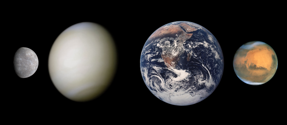
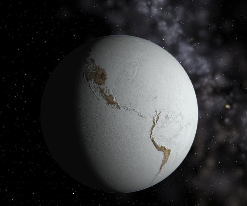
Mercury, Venus, Earth and Mars – Source: NASA, Wikimedia Commons.

One branch of Earth Science in particular has revolutionised geoscientists’ understanding of the interior of the Earth: that branch is seismology.

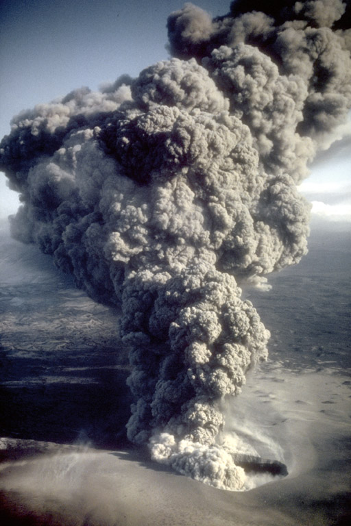
Seismology is the study of seismic waves. In other words, the study of the energy released by earthquakes. Once released, this energy travels in all directions, moving from the ‘source’ point (this can be a natural earthquake or a man-made detonation), through the interior of the Earth, and back up to the surface again.

Seismology is useful because the seismic waves travel differently, and at different speeds, depending on the material they travel through. When a wave reaches a boundary between two different materials or layers within the Earth, it will be deflected: it can either be transmitted to the layer below (but in a slightly different direction), it can travel along the boundary itself, or it can be reflected back to the surface. When a wave passes through the boundary and into the next layer, the amount and direction of the deflection will depend on whether the material below is more or less dense than that above.

Seismic waves travelling through a layer of the Earth – Source: Julia Schäfer, Wikimedia Commons.

These multitude of possible pathways mean that, by looking at how and where on Earth a seismic wave arrives back at the surface, scientists can take a good guess as to what it has travelled through. By building up this information for more and more waves, they can start to paint a good picture of what is going on beneath our feet. Studying seismic waves for geoscientists is a little bit like carrying out a CAT scan for doctors: it allows them to scan the interior of something they cannot see from the outside.

Seeing to the centre of the planet

For my ‘Momentous Discovery in Geology’, I chose to look at a huge moment in the history of seismology: the discovery of the Earth’s inner core. And along with a momentous discovery, comes a momentous discoverer: Danish seismologist Inge Lehmann.

Internal structure of the Earth – Source: Kelvinsong, Wikimedia Commons.

The Earth is a little bit like an onion, in that it has layers. The outermost layer, which we live on, is called the crust. It can be as thin as a 10 kilometres under the oceans and as thick as 70 kilometres under large mountains such as the Himalayas.

Below the crust is the mantle, which makes up over 80% of our planet’s volume. The mantle is mainly solid but can behave in a viscous way when deformed very slowly, over geological timescales.

At the centre of the Earth lies the dense, metallic core. It is predominantly made of iron and nickel. The outer part of the core is liquid and plays an important role in influencing the Earth’s magnetic field.

The core lives nearly 3000 km beneath the surface and has a temperature of nearly 6000°C. It is too deep, too hot and too far to explore with any kind of instrument. This is where seismology steps in.

A liquid ball of molten metal?

Towards the beginning of the 20^th century, seismologists realised that the core must be liquid, thanks to the precious seismic waves they were observing.

When an earthquake occurs, energy is released in the form of two distinct types of seismic waves. Surface waves travel, as their name suggests, along the surface of the planet. These are the waves that cause the damage to human life and infrastructure. Body waves, on the contrary, travel inside the Earth and get deflected by the different layers they travel through, depending on whether each layer is more or less dense than its predecessor.

P- and S-waves travelling through a medium – Source: Actualist, Wikimedia Commons.

Body waves can be further split into two types, distinguishable by the way in which they displace the medium they travel through: Primary waves, or P-waves, and Secondary waves, or S-waves.

These two wave types travel differently through the Earth. One of the important characteristics of S-waves is that they cannot travel through liquid. P-waves can do but slow down considerably when not travelling through solid material.

These properties are what alerted scientists that there was something molten down in the centre of the Earth:

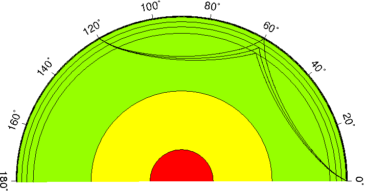
When seismic waves are released from an earthquake, they travel in all directions and should therefore be able to reach back to the surface all around the planet. However, seismologists noticed that seismic waves generated by an earthquake somewhere on the surface of the planet were not being observed at every seismometer on the surface. This no-wave zone is what is called the P- or S-wave shadow zone, where no arrivals can be recorded for a given earthquake.

Paths of P- and S-waves through the Earth's core: the liquid outer core cases a shadow zone - Source: USGS, WIkimedia Commons.

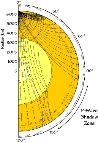
Paths of P-waves through the Earth’s core: the liquid outer core causes a shadow zone – Source: USGS, Wikimedia Commons.

The presence of this shadow zone meant that our P- and S-waves must be affected by something liquid, deep inside the Earth. And so arose the hypothesis of a liquid core.

Something more to the story

In 1929, a large earthquake occurred near New Zealand. Seismologists were quick to study the seismic wave arrivals at seismic stations around the world but Inge Lehmann studied them a little more closely than her peers.

She was puzzled by what she saw: seismometers located within the P-wave shadow zone of the earthquake, where no arrivals should be recorded, were showing signs of the earthquake’s waves. If the core was one large ball of liquid material, this should not be possible.

Lehmann suggested that these waves had travelled some distance inside the liquid core before bouncing off some other, previously unknown, boundary. This bouncing deflected the waves in another direction and meant that they found themselves arriving within the shadow zone.

This hypothesis was the basis of careful studying by Inge Lehmann of more seismic arrivals around the world and she eventually published her results in her revolutionary 1936 paper P’ (or P-prime). Today, the boundary between the outer and inner core is commonly known as the ‘Lehmann discontinuity’.

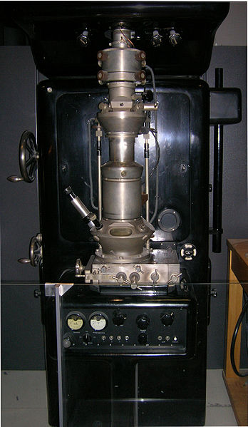
Inge Lehmann’s theory was later confirmed with the development of more sensitive instruments.

Lehmann was a pioneer in the world of seismology and among women scientists, establishing a new theory about the Earth in a very much male-dominated world.

In 1971, the American Geophysical Union awarded her the William Bowie medal, its highest honour. Inge Lehmann went on to live to the age of 105 and published her last paper in 1987, at the age of 99.

A momentous discoverer and scientist indeed.

Momentous Discoveries in Geology – The World of Nano!

Flo Bullough September 27, 2013

I first came across the intriguing world of nanoparticles when I saw an awe-inspiring talk by nano-extraordinaire Professor Michael Hochella from Virginia Tech at the Geological Society. He wove a fascinating tale about the world at nanoscale, the special properties, the infinite uses and the potential environmental impacts as well as outlining the need for caution, scrutiny and intensive research from the scientific community in the wake of an exploding nanotechnology industry. I’ve decided to re-visit the area of nanoscience for the ‘Momentous Discoveries in Geology’ blog festival.

What’s so special about Nanoparticles?

Solutions of gold nanoparticles of various sizes. The size difference causes the difference in colors. Source – Aleksander Kondinski, Wikimedia Commons.

Nanoparticles refer to particles between 1 and 100 nanometers in size and can be found in nature, inadvertently produced by humans or most recently, manufactured as part of the boom in nanotechnology. Their geo-relevance comes from both their behaviour in nature and potential nanotoxicity but also in their manufacture for engineering processes such as environmental tracers and remediation materials. Nanoparticles are unique and special in their physical properties, which can vary greatly from macro-scale properties. Nanotechnology exploits these unusual properties to improve the efficiency and sustainability of already existing processes. They are highly mobile, have enormous specific surface areas, unexpected optical properties and can exhibit what are known as quantum effects. An example being: superparamagnetism (magnetization that can randomly flip direction under the influence of temperature) a characteristic found in ferromagnetic materials smaller than 10nm. Nanoparticles can also have unusual optical properties: gold nanoparticles for example appear deep red to black in solution, depending on their size. They also melt at much lower temperatures (~300 °C for 2.5 nm size) than gold slabs (1064 °C). Their first known use for their colour-changing properties was back in roman times (30BC – 640AD), using gold nanoparticles, which were impregnated into the glass of

The Lycurgus Cup – a 4th-century Roman glass cage cup , which shows a different colour depending on whether or not light is passing through it; red when lit from behind and green when lit from in front due to the incorporation of nanoparticles – You can go and see it in the British Museum! Source – Johnbod, Wikimedia Commons.

goblets to give a colour change from green to blood red when lit from behind. The requirement of the exact mixture of sizes to manifest this effect suggested that the Romans knew what they were doing!

Early history of nanoparticles

The discovery of nanoparticles has not so much happened as a single momentous discovery but as a series of moments over a ~100 year period. As with many discoveries, they are as a result of breakthroughs in instrumentation and technology which breakdown the barrier to discovery. In addition to the early use in roman times, nanoparticles were also used in the medieval (500-1450AD) and renaissance (1450-1600 AD) periods, again for their colour-changing properties for use in stained glass windows in medieval times and for colouring ceramics during the renaissance. The deep reds you see are caused by the incorporation of gold nanoparticles in the glass and the deep yellows are caused by silver nanoparticles. We also see this effect used in Ceramics. In the Islamic world, where the incorporation of gold in artistic representations was not allowed, the solution was using dense nanoparticulated layers of glaze to generate a golden metallic shine. This colour changing capacity is caused by the size of the materials that are incorporated. Photography is also an early example of nanotechnology which is reliant on the production of silvernanoparticles that are sensitive to light.

When were they discovered?

Michael Faraday – 1861. He first described the optical properties of gold nanoparticles in his classic 1857 paper. Source – Wikimedia Commons.

The earliest and most significant breakthrough came during Michael Faraday’s pioneering experiments and his seminal paper in 1857 where he described the optical properties of nanometer-scale metals for the first time. He prepared the first metallic colloids (fine particles that suspend in solution, in between dissolved and settling particles, size range between 2-500 nm). He saw that they had special electronic and optical properties and stated – “It is well known that when thin leaves of gold or silver are mounted upon glass and heated to a temperature which is well below a red heat (~500 °C), a remarkable change of properties takes place, whereby the continuity of the metallic film is destroyed. The result is that white light is now freely transmitted, reflection is correspondingly diminished, while the electrical resistivity is enormously increased.”.

348px-Ernst_Ruska_Electron_Microscope_-_Deutsches_Museum_-_Munich-edit

First Electron Microscope with resolving power higher than that of a light Microscope designed by Ernst Ruska in 1931 with a magnification of around 12,000 times. Source – J Brew, Wikimedia Commons

While the unusual and fascinating properties of nanoparticles had been described, they were still too small to be seen and it took another 84 long years before electrical engineer Max Knott and physicist Ernst Ruska constructed the prototype electron microscope in 1931. This breakthrough put a spotlight on the “small world” and was an important step in allowing research at the nanoscale. This was followed by Erwin Mueller’s field-ion microscope which allowed the viewer, for the first time in history to observe individual atoms and their arrangement on a surface. This was a landmark invention allowing magnification of more than 2 million times. These technological developments formed the foundation for many other nano breakthroughs to come such as the ‘tunneling phenomenon’, the development of the field of molecular electronics, the development of Surface Enhanced Raman Spectroscopy (SERS), instrumental in the field of nanotechnology, the buckyball, quantum dots (which have implications for how solar energy is collected) and carbon nanotubes.

_____________________________________________________________________

This post is for a geoscience blog carnival called The Accretionary Wedge, which is being hosted by Matt Herod and you can see the call for posts here.

Climate change: it’s just a matter of time!

Marion Ferrat September 20, 2013

Natural or man-made: what factors are responsible for the climate changes we are seeing today? Ahead of the release of the latest IPCC report next week, Marion Ferrat discusses the different factors affecting climate change and shows that who takes the blame all depends on timing…

Over the past century, our planet’s climate system has been changing. Changes in the composition of the atmosphere, holes in the ozone layer, warming temperatures and sea level rise are only some of the factors that have been observed worldwide.

Earth taken by the crew of the Apollo 17 spacecraft – Source: NASA, Wikimedia Commons.

A fixed observer looking at our planet for the past few billion years would have seen patterns of warming and cooling of its surface, ice sheets growing to the tropics or shrinking to the tips of the poles, deserts forming, seas drying, oceans overturning and vegetation changing. So who is to blame for our current changing climate? Is climate change natural or man-made?

What factor is most important in driving climate change really depends on the timescale you consider. So let’s take a short journey through climate space and time to shed more light on who is to blame for climate change.

The million-year climate change: blame the continents
The hundred thousand-year climate change: blame the Sun
The thousand-year climate change: blame the climate!
The 21st century climate change: blame ourselves

The million-year climate change: blame the continents

The Earth’s climate history is divided into primary climate periods, millions of years long, of increase or decrease in the temperature of the Earth’s surface and atmosphere. These periods are referred to as Greenhouse Earth and Icehouse Earth (or Ice Age), respectively.

Fictional representation of a ‘Snowball Earth’ – Source: Neethis, Wikimedia Commons.

The main characteristic of an Ice Age or Icehouse world is that permanent ice sheets are present at the surface of the Earth. The thick ice sheets covering Greenland and Antarctica today mean that we are currently living in an ice age, which began 2.6 millions of years ago.

In a Greenhouse world, on the contrary, ice sheets and glaciers are absent from the surface of the Earth. At the height of these times, carbon dioxide levels in the atmosphere can vary between a few to a few hundred times their present level.

The exact causes behind shifts between greenhouse and icehouse worlds are still debated but scientists agree that two factors play an important role: the position of continents at the surface of the Earth and the concentrations of greenhouse gases (mainly CO2 and methane) in the atmosphere.

Animation of the breakup of Pangea – Source: USGS, Wikimedia Commons.

The position of the continents and oceans is important in driving the million-year-long climate cycles as it has a huge influence on atmospheric composition and oceanic flows (see this cool animation showing the movement of the British Isles over geological time!). For example, the grouping of continents in particular places can stop the flow of warm water from the equator to the poles and cool down polar water, until ice sheets begin to form.

Eruption column rising from the east Ukinrek Maar crater in Alaska - Credit: R. Russell/USGS, Wikimedia Commons.

Eruption column rising from the east Ukinrek Maar crater in Alaska – Source: R. Russell/USGS, Wikimedia Commons.

Plate tectonics can also drive climate change by influencing the concentration of CO2 in the atmosphere. The presence of large volcanoes can play an important role in driving long-term shifts from an icehouse to a greenhouse world because extensive volcanism can release large quantities of greenhouse gases into the atmosphere. Once enough CO2 builds up, the greenhouse effect kicks in and acts to warm the planet, pulling it out of its million-year ice age.

Once an initial change is triggered, the climate system will act to amplify it internally until the switch between ice and greenhouse world is complete.

The hundred thousand-year climate change: blame the Sun

Overlain on top of the huge greenhouse or icehouse periods are shorter, regular periods of climate change.

Over timescales of tens to hundreds of thousands of years, the Earth undergoes cycles of cooling and warming, driven primarily by small changes in the amount of energy received from the Sun. These periods are known as glacial and interglacial cycles, i.e. times within an ice age when the Earth is colder or warmer than average. We are currently living in an interglacial period called the Holocene, which began roughly 11,000 years ago.

An example of changes in eccentricity.

Glacials and interglacials are driven by what we call orbital changes: small changes in the Earth’s orbit, which alter the amount of solar energy received at the Earth’s surface. These changes are cyclical and known as Milankovitch cycles, after the Serbian astronomer who first recognised them during the First World War.

Obliquity or axial tilt – Source: Dna-webmaster, Wikimedia Commons.

There are three types Milankovitch cycles. The first, called eccentricity, is linked to the shape of the Earth’s orbit around the sun. The orbit changes from the shape of a circle to that of an ellipse over average timescales of roughly 100,000 years. When the orbit is more elliptical, the Earth is either closer or further away from the Sun than when the orbit is circular, driving changes in the amount of solar energy received at the surface. Climate data for the past 800,000 years show that ice sheets have grown and shrunk roughly every 100,000 years, likely driven by changes in eccentricity.

Precession of Earth’s rotational axis due to the tidal force raised on Earth by the gravity of the Moon and Sun – Source: NASA/Mysid, Wikimedia Commons.

The second type is linked to changes in the Earth’s axis. The Earth rotation axis is tilted; this tilt is largely what drives our seasons. The amount of tilt (or obliquity) also varies with time, over periods of roughly 41,000 years.

Finally, if one could watch the Earth from a fixed star in the universe, they would see its axis rotating slightly, a little bit like the wobble of a spinning top as it slows down. This is called precession and changes over periods of roughly 23,000 years.

The 100,000, 41,000 and 23,000-year Milankovitch cycles alter the amount of sunshine received on Earth and drive many changes in the Earth’s climate on these timescales, as has been observed in temperature and CO2 records.

The thousand-year climate change: blame the climate!

X-ray photo of surface sediment (0-25 cm) from the Southern Ocean with scattered gravel as ice rafted debris – Source: Hannes Grobe/AWI, Wikimedia Commons.

In the last decades of the 20^th century, scientists began to find clues in the geological records of the North Atlantic Ocean and Greenland ice sheet that climate change was also occurring at higher frequencies than those linked to orbital and tectonic cycles.

Icebergs contain plenty of eroded rock and sediment. When they break-off into the ocean and melt, much of this material falls to the seafloor and can be seen as anomalies in the geological record called ice-rafted debris. Ocean cores revealed that thousand-year pulses of such debris could be found regularly throughout the past 100,000 years, suggesting rapid periods of iceberg break-off and discharge of cold water to the North Atlantic Ocean.

The Greenland ice cores also revealed that periods of rapid warming followed by slow cooling were occurring every few thousand years. These events seem to occur roughly every 1,500 years, though precise dating on these timescales can be difficult.

Such events are known as millennial cycles and are what scientists refer to as ‘abrupt’ climate change.

Similar changes have since been recognised in many locations, including the north Pacific Ocean and the tropics, suggesting that changes can be rapidly transferred between different regions of the globe by the climate system itself. One possible mechanism is that large bursts of cold water in the North Atlantic Ocean could alter the global circulation of ocean currents, which is largely driven by density changes in the North Atlantic region.

The global circulation of the oceans, known as the ‘conveyor belt’ – Source: Thomas Splettstoesser, Wikimedia Commons.

The 21st century climate change: blame ourselves

So Earth’s climate has changed drastically throughout the course of its history, driven by external factors such as changes in the Earth’s orbit and internal factors such as tectonics and physical connections between different parts of the climate system. Yes, these climate changes are natural and, yes, temperatures and CO2 have at multiple times been higher than they are today.

However, there are a few points worth making:

Smog over Beijing, China.

#1 – The most drastic changes have occurred very slowly, on timescales of hundreds of thousands to millions of years. These are thousands of orders of magnitude larger than that of a human life;

#2 – At all scales, atmospheric CO2 concentrations have played a huge role in climate change, contributing largely to the greenhouse effect, affecting ocean composition and acidity and being a crucial component of plant and animal life cycles;
#3 – Until the start of the industrial revolution, humans in our modern societies have evolved and lived through relatively stable climate conditions , with stable CO2 concentrations between 260-280 parts per million (ppm) for the past 10,000 years;
#4 – CO2 levels have constantly increased since the industrial revolution due to human emissions. A record global atmospheric CO2 concentration of 400 ppm was observed in May 2013 at the Hawaiian Mauna Loa observatory. This is the highest CO2 level in over 800,000 years, higher than any other interglacial period during this time.

Atmospheric CO2 during the past 417,000 years (417 kyr). Blue: CO2 records from ice cores drilled at the Vostok station in Antarctica; Red: CO2 increase to 380 ppm between 1800 and today due to anthropogenic emissions from fossil fuels- Source: Hanno, Wikimedia Commons.

Atmospheric CO2 during the past 417,000 years (417 kya). Blue: Records from ice cores drilled at the Vostok station in Antarctica; Red: CO2 increase since 1800 due to anthropogenic emissions from fossil fuels – Source: Hanno, Wikimedia Commons.

The speed at which this human-induced rise in CO2 has occurred is worrying, increasing by nearly a third in just over 150 years.

The climate system will adjust to these changes over the next centuries as it has in the past. But the real issue is that these adjustments will not be in line with our modern inhabited world. As millennial cycles have shown, polar changes can be transferred between different regions of the Earth in ways that we still do not fully understand. Humans as a whole will likely adapt to future climate repercussions but particular vulnerable regions and communities will not.

Atmospheric CO2 concentrations measured at Mauna Loa, Hawaii - Source: Robert A. Rohde, Wikimedia Commons.

Atmospheric CO2 concentrations measured at Mauna Loa, Hawaii, since 1960 – Source: Robert A. Rohde, Wikimedia Commons.

Modern climate change is not a case of the end of the world but more of the end of the world as some people know it. Small islands and low-lying regions will suffer, so will areas affected by unpredictable droughts or floods.

By contributing in such an excessive way to concentrations of atmospheric CO2, humans are to blame for the climate changes we will continue to see in coming decades and even centuries; and not all of us will be able to adapt to it.

What’s all the Phos about?

Flo Bullough September 12, 2013

Phosphate use for fertilisers, essential in modern agriculture, is hitting an all time high while resources are being heavily depleted. Flo discusses the background, numbers, geopolitics and potential solutions behind the issue of ‘the end of phosphorus’.

The Issue

Modern agriculture has developed in-line with the availability of high quality phosphate-rock fertilisers. Source – João Felipe C.S, Wikimedia Commons.

The dilemma over diminishing natural resources is a topic of our times with the daily bulletins filled with reports related to resource shortages. These mainly focus around water, energy and food which are imperative for human survival. Whilst energy and water are often debated in the media and political chamber, an area that gets much less attention is agriculture, and in particular diminishing phosphate resources used for industrial fertiliser. Modern agriculture, particularly in developed countries has used mined phosphate for fertilisers for decades but this finite resource is being depleted at an alarming rate.

A combination of growing population, aspirational lifestyles and the demand for phosphate-intensive meat and crops has caused the rapid reduction of phosphate rock resources. In the past, prior to the advent of phosphate mining, additional phosphate for farming and agriculture was sourced from manures

Prior to use of phosphate rock, it was replenished through the use of manure. Source – Malene Thysson, Wikimedia Commons.

and organic waste, but as agriculture intensified, the hunt for easier, more accessible phosphate began. From the mid-20th century onwards, the use of rock phosphate was used as a high quality, easily accessible sources of phosphorus which gave rise to the modern fertiliser industry as we see it today. Farmers in rich countries such as Europe and North America became hooked on the cheap and easy phosphorus which readjusted agriculture practices and set phosphate demand through the roof.

Background

Phosphorus (P) is a non-metallic element which is almost always present in a maximally oxidised state (PO₄^3-) as inorganic phosphate rocks due to its reactivity. Elemental phosphorus can exist as red and white (known for its use in weapons and artillery) phosphorus but almost never found as a free element in nature.

It is one of the building blocks of life and life simply wouldn’t exist without it. It is a key component of DNA, RNA, ATP and phospholipids and is essential to cell development, reproduction and in animals, bone development. The use of phosphorus compounds in fertilisers is due to the need to replace the phosphorus that plants remove from the soil.There is no substitute for this element. Supplies are limited and much is currently wasted, creating concerns about future supplies in the EU and worldwide.

Peak Phosphorus?

A graph of world phosphate rock production vs. year from 1900-2009 obtained from the U.S. Geological Survey. Source – Thomas D. Kelly and Grecia R. Matos, Wikimedia Commons.

Recently there has been a proliferation of articles and discussion over the potential for ‘peak phosphorus’ in the next 20-30 years. World production recently peaked at <160 million metric tonnes (mmt) in 2008. Whilst the majority of people agree that phosphorus is a resource that is of concern, not everyone agrees with the peak phosphorus hypothesis or its potential timing. Proponents of the argument include this group of academics who published a paper entitled ‘The story of phosphorus: Global food security and food for thought’ and Jeremy Grantham, co-founder of the investment firm Grantham, Mayo, Van Otterloo, who recently wrote a piece in Nature. On mined-phosphate fertilisers, Jeremy Grantham stated that ‘There seems to be only one conclusion: their use must be drastically reduced in the next 20–40 years or we will begin to starve’. Much of the peak phosphorus argument comes from a widely produced diagram from a 2009 paper in Global Environmental Change depicting peak phosphorus to be around 2030 followed by production declining at an accelerating rate. Detractors to this theory say that the markets are likely to adjust to this problem and cause the price to rise thus forcing a reduction in use and a push for technology to advance to find new sources or recycle current phosphate use. The International Fertiliser Development Center (IFDC), through extensive data gathering state that there is “no indication that a “peak phosphorus” event will occur” in the next 20-25 years.

Resources and Geopolitics

Phosphate mine near Flaming Gorge, Utah. The large size of phosphate mines is dictated by the dispersed nature of phosphate in the rock. Source – Jason Parker-Burlingham, Wikimedia Commons.

Phosphate rock is typically mined at high volume due to its dispersed nature in the rock. Phosphate, in the mineral form of apatite in phosphate rock, is not bioavailable to plants and must be processed to convert it to a plant-available form. The concentrate is used to produce phosphoric acid which is then used in fertiliser products. Phosphate rock can come in either a sedimentary or igneous form, with sedimentary making up >80% of total global production.

Topographic map of Western Sahara. Western Sahara is disputed territory but is currently controlled by Morocco and therefore the Moroccan Royal Family. Source – Sadalmelik, Wikimedia Commons

In addition to the concern over the amount of resources and rate of use, also of concern is the location of much of the world’s supplies. Europe in particular has scant phosphate resources with a small amount in Finland. According to the IFDC report from 2010, 72.1% of the world’s phosphate rock production was accounted for by China ( 31.5%), U.S.A (18.7%), Morocco and Western Sahara (15.5%) and Russia (6.4%). However a significant proportion of the world’s high-grade supplies are located in the disputed territory of Western Sahara in North-West Africa, currently controlled by Morocco. This has been termed by Jeremy Grantham as ‘the most important quasi-monopoloy in economic history’.

Country	Mine Production 2007	Mine Production 2008	Reserves	Reserve Base (estimated)
China	45,700	50,000	4,100,000	10,000,000
Morocco and Western Sahara	27,000	28,000	5,700,000	21,000,000
Russia	11,000	11,000	200,000	1,000,000
United States	29,700	30,900	1,200,000	3,400,000
World Total (rounded)	156,000	167,000	15,000,000	47,000,000

Table adapted from USGS Mineral Commodity Summaries January 2009. Data is presented in thousand metric tonnes.

Phosphate rock resources in Western Sahara are extremely large and still incompletely explored and therefore it is not understood if the rock is producible at current prices and costs as there is little to no data. The IFDC estimates global resources of 290,000 mmt but if Morocco and Western Sahara resources are included (340,000 mmt) it may increase to 470,000 mmt, as seen in the above table.

Environmental Impacts

800px-EutrophicationEutrophisationEutrophierung

Eutrophication in a pond in Lille, France. Eutrophication is caused by the enrichment of an ecosystem with chemical nutrients such as phosphorus. Source – F. lamiot, Wikimedia Commons.

The use and mining of phosphorus also carries risks. In agricultural use not all of the phosphorus is absorbed by crops which results in leaching into the water. This causes the much discussed eutrophication effect causing algal blooms. Phosphorus mining is also difficult environmentally as it generates a large amount of the waste product phosphogypsum which contains both toxic heavy metals and low levels of radiation. This is very difficult to dispose of and often results in mounds of unprocessed waste material.

As lower-cost phosphate resources will be mined out, mining companies will utilise lower grade ores which will incur the use of more energy and water and will cause the price to go up. Availability of water is of high importance to mining operations and indeed this can dictate the feasibility of phosphate extraction, areas of low water availability may completely restrict development of the mine. Another way in which water, energy and food are interconnected.

What next?

Wastewater discharge pipe – New studies show useable phosphorus can be recovered from wastewater. Source – Department of Agriculture, Wikimedia Commons.

Regardless of the proximity of ‘the end of phosphorus’ it is very much a finite resource and thus development towards more effective use and recycling needs to take place. Recently, the Environment section of the EC launched a consultation into how to use phosphorus in a more sustainable way, following on from a conference held in March on Sustainable Phosphorus. They have also posted a series of informative videos that can be found here. Much work has been done on the ways in which we can curb our phosphate use or recycle it more effectively. More must be done to monitor and reduce phosphate use as well as recycle wasted phosphate. A few of the potential solutions are listed below.

Phosphate reduction

Changes in people’s daily diet away from phosphorus-intensive foodstuffs such as meat.

Since much of phosphorus is lost from the food cycle through waste, a reduction of food waste and its reuse in composts etc could reduce demand.

Current agricultural practices result in a very high use of fertilisers. A switch to techniques and practices that conserve more soil nutrients would go some way to reduce phosphorus waste. This includes organic agriculture and use of permaculture (sustainable and self-sufficient agricultural practices).

Genetic engineering could produce plants that can flourish with much lower phosphorus use.

Recycling

We can recover useable phosphorus from waste streams including urban sewage, since current systems already remove phosphorus from sewage to preserve water quality. Wastewater carries a lot of struvite, a mixture of ammonium, magnesium and phosphate which builds up in the pipework.

A team of canadian researchers believe struvite can be turned into environmental friendly fertiliser, as discussed in this national geographic article. Together with the local government they have set up a lab next to a waste water treatment plant. This process works by altering the pH and allows the wastewater chemical to bond together into pellets through a turbulence process. Currently a working prototype can turn out several tons of pellets a month. Since 2010, the technology has been incorporated into 5 waste water facilities in North America. Whilst there are some cost issues to address, there is relatively little further work required to reproduce this technology on a wide scale. Higher phosphate prices would push wastewater recovery to be economic.