Cryospheric Sciences | Image of the Week – Powering up the ground in the search for ice

Electric Resistivity Tomography profile of the north-facing slope of the Rohrbachstein in canton Bern, Switzerland [Credit: University of Fribourg, Switzerland].

In an earlier post, we talked briefly about below-ground ice and the consequences of its disappearing. However, to estimate the consequences of disappearing ground ice, one has to know that there actually is ice in the area of study. How much ice is there – and where is it? As the name suggests, below-ground ice is not so easy to spot with the naked eye. Using geophysical methods, however, it is possible to obtain a good idea of the presence and whereabouts of ground ice, and of frozen ground, in an area of interest.

Looking for ice

Before starting a geophysical survey, which requires instrumentation and time, you might want to take a look at your area of interest and estimate, whether ice presence is even an option. The first indicator is temperature, which has to be in the favor of permafrost presence. Other indicators for presence are surface features such as mounds that could be caused by considerable frost heave, lobes perpendicular to the slope and front angles exceeding the critical angle of repose. They can indicate that ice has had an influence on the geomorphology in the area.

If you suspect ground ice in your area of interest, and you want to confirm or rule out your suspicion as well as investigate the extent of the ice, you might consider doing a geophysical survey. There are a few useful inherent properties of ice that make it possible to distinguish it from rock, air or water. These properties will determine the choice of geophysical methods to use. This week, we will illustrate two methods which, when combined, can be useful tools for determining ground ice presence or absence. The test subject is an area of suspected frozen ground just below 3000 m altitude – the Rohrbachstein in canton Bern, Switzerland.

Electrical resistivity tomography

In an electrical resistivity tomography (ERT) survey, we measure the potential difference (ΔU) of a material, over a given distance, when applied with a certain current strength (I). From the fact that resistance is computed by dividing U by I, the electrical resistivity of the material can be estimated. The resistivity can be seen as the reciprocal of the material’s electrical conductivity and is measured in mΩ. Practically, an array of electrodes are placed in the ground with a certain spacing and a certain length of the profile. The spacing and length of the profile determine the resolution and penetration depth. All electrodes are then connected with a cable to each other and to the instrument, which works as both a voltmeter and a source of current. Then, systematic measurements of potential difference can be conducted throughout the whole profile.

Water has an electrical resistivity of 10-100 mΩ, whereas ground ice has a resistivity of 10³ to 10⁶ mΩ. This makes this method practical for distinguishing liquid from frozen water in permafrost areas. The resistivity of rock is between 10² to 10⁵ mΩ, and the resistivity of sediment depends on the mixture of rock, water, ice and air. Air has an extremely high resistivity, which should be easy to point out, but since below-ground material is mostly a mixture of all the mentioned components, things are very often more blurry. What one actually looks for in the measurements is areas of higher, lower and in-between electrical resistivity values. An example of such a case is displayed in our Image of the Week.

Our Image of the Week shows the resistivity profile of a slope at just below 3000 m altitude in the Bernese Alps, Switzerland. For comparison, the same slope is shown in a normal photo in Fig. 2 (not to scale). Blue colours mark high resistivities, red mark low, and green mark somewhere in between. From this profile, we might conclude that the upper layers of the lower slope are moist and underlain by bedrock (red and green, respectively, whereas the upper slope seems to be moist below an area of high resistivity (red below green-blue). Additionally, there is a significant feature of high resistivity in the middle of the slope. This slope could contain ice in those blue areas. However, the high resistivities could also be caused by air volume in this blocky site. To be certain, we can use an additional method.

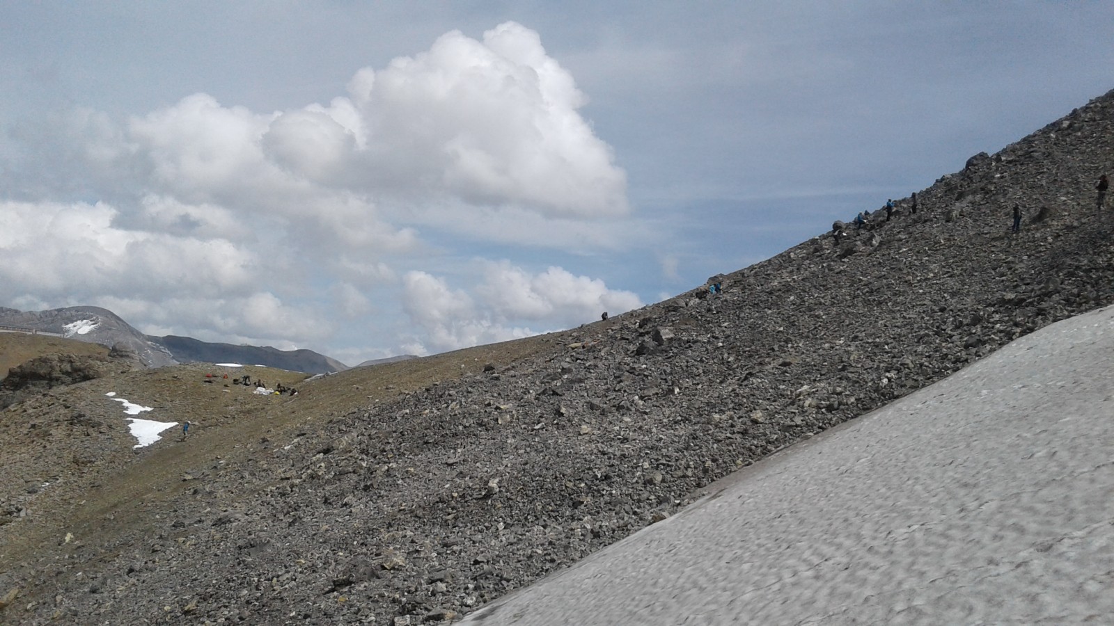
Fig. 2: Photo of the north-facing slope of the Rohrbachstein in canton Bern, Switzerland. The photo was taken facing east and shows the upper part of the slope analyzed with ERT and seismic refraction, but is not to scale compared with the Image of the Week and Fig.4 [Credit: Laura Helene Rasmussen].

Seismic refraction analysis

To distinguish air from ice, we can do a survey of the subsurface using seismic refraction analysis. Seismic refraction surveys use the fact that the speed (in ms^-1) of sound wave propagation is different through different materials. The speed is estimated by placing geophones in a profile line and creating a sound wave by hitting the ground with a sledgehammer in between them (Fig. 3). The geophones detect the sound wave from this hammer blow one by one as it travels through the subsurface, and the time it takes for each geophone to receive the signal is noted. This allows us to calculate the seismic (sound) velocity from the distance and travel time. Different layers in the subsurface with different properties, and thus different seismic velocities, will cause the sound wave arriving at their surface to be refracted with different delay compared to the direct wave (which travels straight from the hammer to each geophone), and that fact can reveal properties of below-ground material.

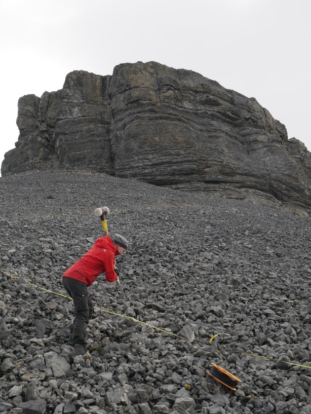
Fig. 3: Hammer-swinging doing a seismic refraction profile [Credit: Hanne Hendricks].

The advantage of this method for ground ice studies is that ice has a seismic velocity of about 3000 ms^-1, whereas sound waves move through air with only 330 ms^-1. Thus, a rough profile of that same slope from our Image of the Week and Fig. 2 using seismic refraction geophysics looks like Fig. 4.

In this profile, red colours denote high seismic velocities and blue colours are very low seismic velocities. The high-resistivity feature in the middle of the ERT profile at about 3-4 m depth, which could contain air or ice, would cause red-purple colours (high velocities) if the feature contained ice, and blue colours (low velocities), if it was air volume. As seen from Fig. 4, colours at depths are reddish and certainly not blue, which makes it likely that the ERT feature at 3-4 m depth is actually an ice body. The high-resistivity area in the surface layers of the upper profile, however, corresponds to the blue colours in this seismic refraction profile, and with high resistivity, but low seismic velocity, this area is most likely air volume and not ground ice.

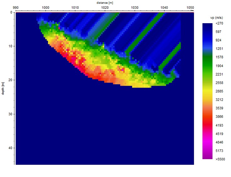
Fig. 4: Seismic refraction profile of the north-facing slope of the Rohrbachstein in canton Bern, Switzerland [Credit: University of Fribourg, Switzerland].

The method depends on the setting

Ground ice does, obviously, come in different forms in different environments, and so the methodological considerations when using geophysical techniques vary in different settings. In this case, we look for ice in a blocky slope. That type of setting presents challenges such as contact problems between sensors and the ground, which can impede the measurements. That issue would not worry a scientist mapping ground ice in a moist Arctic lowland site. The lowland scientist might, however, have to consider resolution issues or salt content in her soil solution when evaluating the results. Perhaps she wants to combine with yet other methods such as drilling permafrost cores for detailed information on ice- and sediment type. As non-destructive methods, covering relatively large spatial areas without having to get a drill rig to the high mountains or a remote Arctic area, however, geophysics can be a good option for ground ice detection.