Do Beers Go Stale in the Arctic? – Jakob Sievers

A curious polar bear investigates an instrument tower on sea-ice. Photo: Jakob Sievers.

A story about CO₂ -fluxes between sea-ice and the atmosphere

What’s it all about?

Whenever I have had to describe my PhD research project to people outside of my research community, I have always found it useful to use an analogy most people are familiar with, namely beers. Now that I have the full attention of the entire class, allow me to explain. Say you were to find yourself at an outside café, grabbing a beer in the beautiful weather with your friends. You get caught up in the conversation and soon your beer is lukewarm and stale and you struggle with the last few drops while gesturing somewhat frantically at the waitress to bring you a new beer. What has happened? Well, the partial pressure of CO₂ (pCO₂) in the beer is much larger, relative to that of the atmosphere. This leads to gradual diffusion (or flux) of CO₂ from the surface of the beer into the atmosphere, and eventually the establishment of an equilibrium pCO₂ in the beer, similar to that of the atmosphere. Of course, you have probably been waving at the waitress long before the equilibrium is reached. Now imagine that you had performed this experiment in the cold of winter. The waitress brings you a beer and from the moment it reaches your table a thin layer of ice starts forming on the top. What happens with the CO₂ levels now?

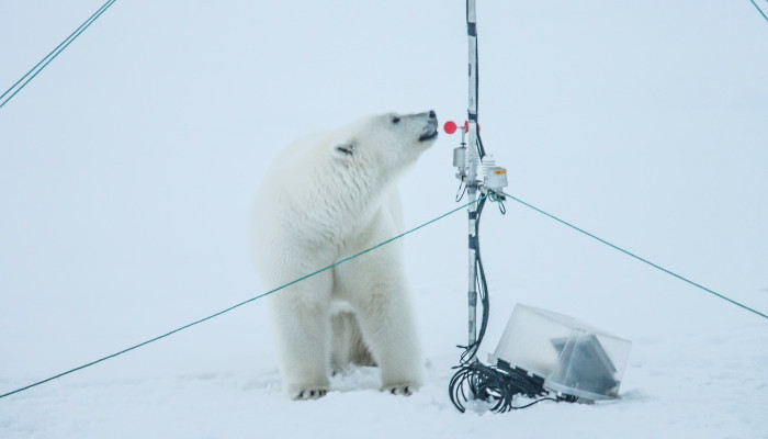
Though a bar would probably have been a nice place for fieldwork, obviously my fieldwork took place in a much colder environment, namely the arctic sea-ice in northeast Greenland. The kingdom of the sort of curious four-legged fella shown in the photo above. And the answer to the above question might be “nothing” in the case of a beer. I.e., the ice works as a sort of lid on the beer, preventing any fluxes of CO₂ from occurring, but what about in a sea-ice environment? Until very recently the beer analogy would have applied equally well here, as most scientists would have told you that no CO₂ fluxes could take place in this sort of environment. Accordingly, all climate models currently treat sea-ice covered regions as regions of no exchange in terms of CO₂. Lately, however, a number of papers have been published, suggesting that fluxes can occur at different stages of the annual sea-ice cycle. The paradigm shift occurred when it was discovered that CO₂ may be transported through brine channels within the sea-ice. Brine channels form within sea-ice because of the salt in the sea-water, and they tend to be larger if the temperature is higher. So, at the bottom of the ice where the ambient temperature is a balmy 0°C, the channels are largest (Fig. 1).

Figure 1: An actual photo of brine channels within sea-ice [Junge et al., 2001, Annals of Glaciology]

It is thought that the bulk of fluxes occur primarily in the spring during sea-ice melting. To understand why, we have to go back to when the sea-ice is formed during wintertime. As the ice forms, salts and CO₂ are concentrated in the brine channels, and are expelled into the ocean through the larger brine channels in the bottom of the ice. The process is called gravity drainage and refers to the sinking of the highly saline and cold brine water which is denser relative to the underlying sea-water. Some of the expelled CO₂ will continue to the deeper ocean column and as such lead to a CO₂ loss of the original surface system. Hence, upon springtime melting, the upper water column has less CO₂ than the atmosphere, which then causes an uptake of CO₂ from the atmosphere. I.e.: a re-carbonization of the beer, so to speak. The mechanism has been coined the sea-ice driven carbon pump and has been estimated to drive an annual uptake of 50 million tons of carbon annually in the arctic alone, constituting a significant fraction of the total CO₂ uptake of the arctic ocean which is estimated to be 66-199 million tons of carbon annually. Hence, understanding the impact of this carbon pump is important, particularly because the impact of climate change is felt more dramatically in the arctic compared to the rest of the world. Sea-ice cover is becoming increasingly ephemeral and glacial freshwater runoff, which inherently has a low partial pressure of CO₂, is becoming increasingly ubiquitous in the fjord systems.

What are the challenges in this field of study?

To incorporate the carbon pump into existing climate models we need first to understand the physical and biogeochemical processes which drive sea-ice carbon fluxes in both coastal and open water conditions as well as during the entire life-cycle of sea-ice. Sounds simple, right? Of course not. Like most experimental investigators in cryospheric sciences we are struggling with considerable logistical challenges in a vast and unforgiving environment, where temperature conditions often have instrument-developers shaking their head in disbelief. “We didn’t test the instrument for that sort of thing”. How reassuring. Secondly, there are substantial risks involved, both for people and instruments, when conducting experiments during periods of thin sea-ice, which also happen to be the periods in which fluxes are most pronounced, and thus all the more important to understand. Fortunately we are equipped with fairly unique vehicles for transportation during these conditions (Fig. 2). Finally, the fluxes that are reported on sea-ice are often significantly smaller than what is typically reported in terrestrial environments, leaving investigators at times struggling to discern actual measurements from artificial noise.

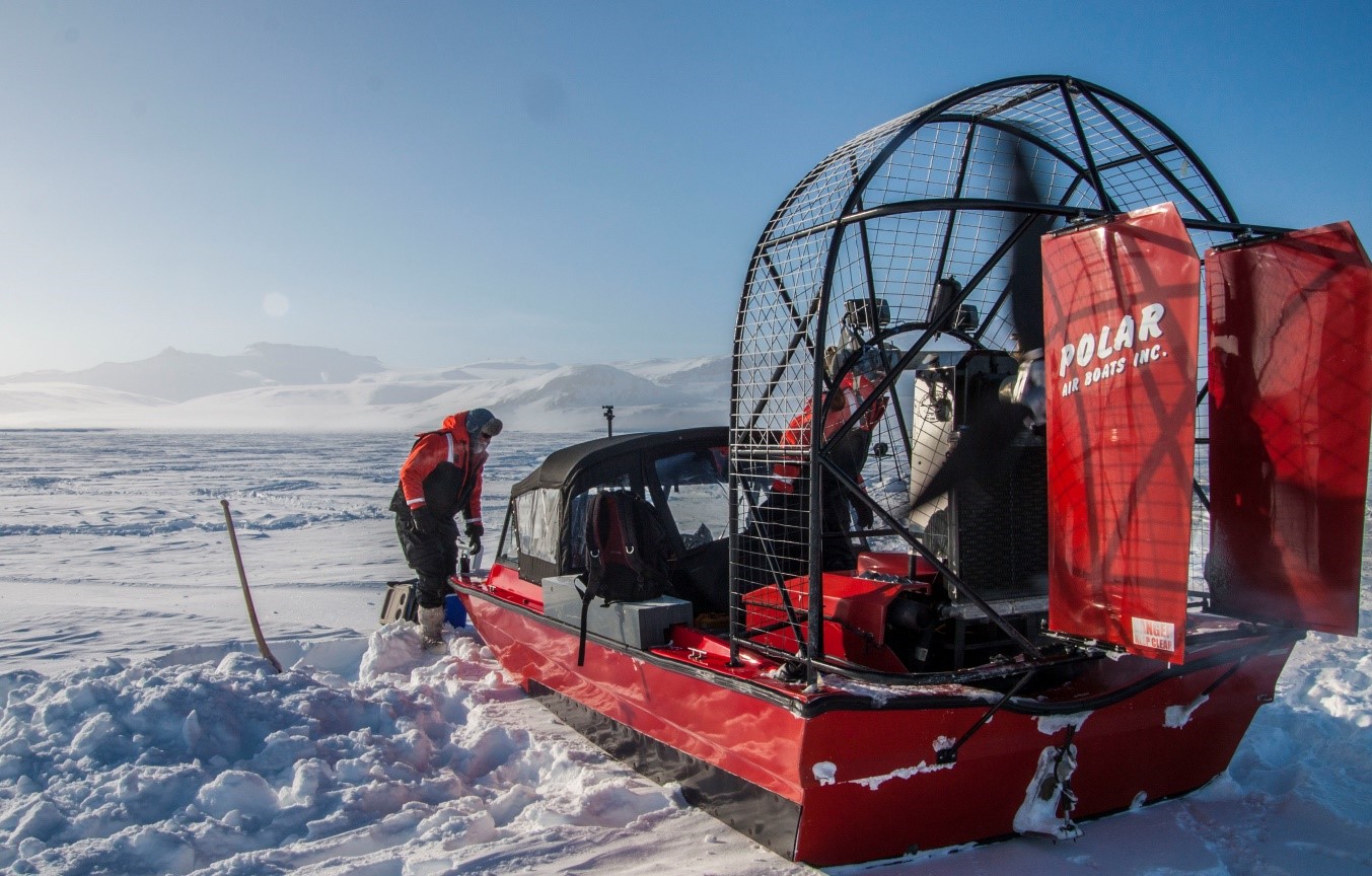
Figure 2: Our polar air-boat for safe and fast transportation on thin sea-ice. During the experiment this bad boy was typically referred to as a gasoline-to-noise converter. In this particular picture the air-boat is pictured on thick sea-ice, hence the use of normal winter clothing instead of marine safety suits. Photo: Jakob Sievers.

What did I focus on during my PhD?

A common method for flux-observation is the micrometeorological Eddy Covariance method. It involves setting up a 2-5m high tower on a surface of interest and at the top installing:

(1) A three-dimensional ultrasonic anemometer, which measures 3D wind patterns,

(2) A gas analyzer, which measures the atmospheric concentration of e.g. H₂O, CO₂ or CH₄ depending on which type of flux you are interested in.

Figure 3: Our eddy covariance tower on thin ice (20cm) in the outermost region of Young Sound (NE Greenland). Photo: Jakob Sievers.

Together they allow for calculation of the average flux in an upwind area in front of the tower. This area will vary in size depending on the height of the tower and wind-conditions. One of our instrument towers are shown in Fig. 3. From a mathematical standpoint the method is very simple, but it requires a number of quite complicated assumptions concerning the characteristic wind-patterns of the environment in question. Often these assumptions are not discussed in detail in papers. During my PhD I found that because most fluxes in a sea-ice environment are so small the critical assumptions began breaking down. It seemed that nearly all observations reflected large-scale meteorological patterns and flow-characteristics of the topography instead of fluxes in the local area of interest. Realizing this, I successfully developed and tested a very comprehensive data-analysis method to disentangle contributions of interest and contributions which were not reflective of the local environment of interest. Due to the technical nature of this new method I will not elaborate here, except to say that it was recently published in the Journal of Atmospheric Chemistry and Physics. Subsequently I was able to analyze simultaneous observations of CO₂-fluxes and environmental parameters such as site energy balance and wind-speed to achieve a better understanding of some basic causal relationships for CO₂ fluxes in a sea-ice environment.

Because this field of study is so new, and in-situ experiments are so challenging, much work is still needed but hopefully we will soon have a sufficiently detailed understanding of the physical and biogeochemical factors driving CO₂ fluxes in the sea-ice environment, to be able to develop a model relationship and upscale that to all polar regions in which sea-ice exist.

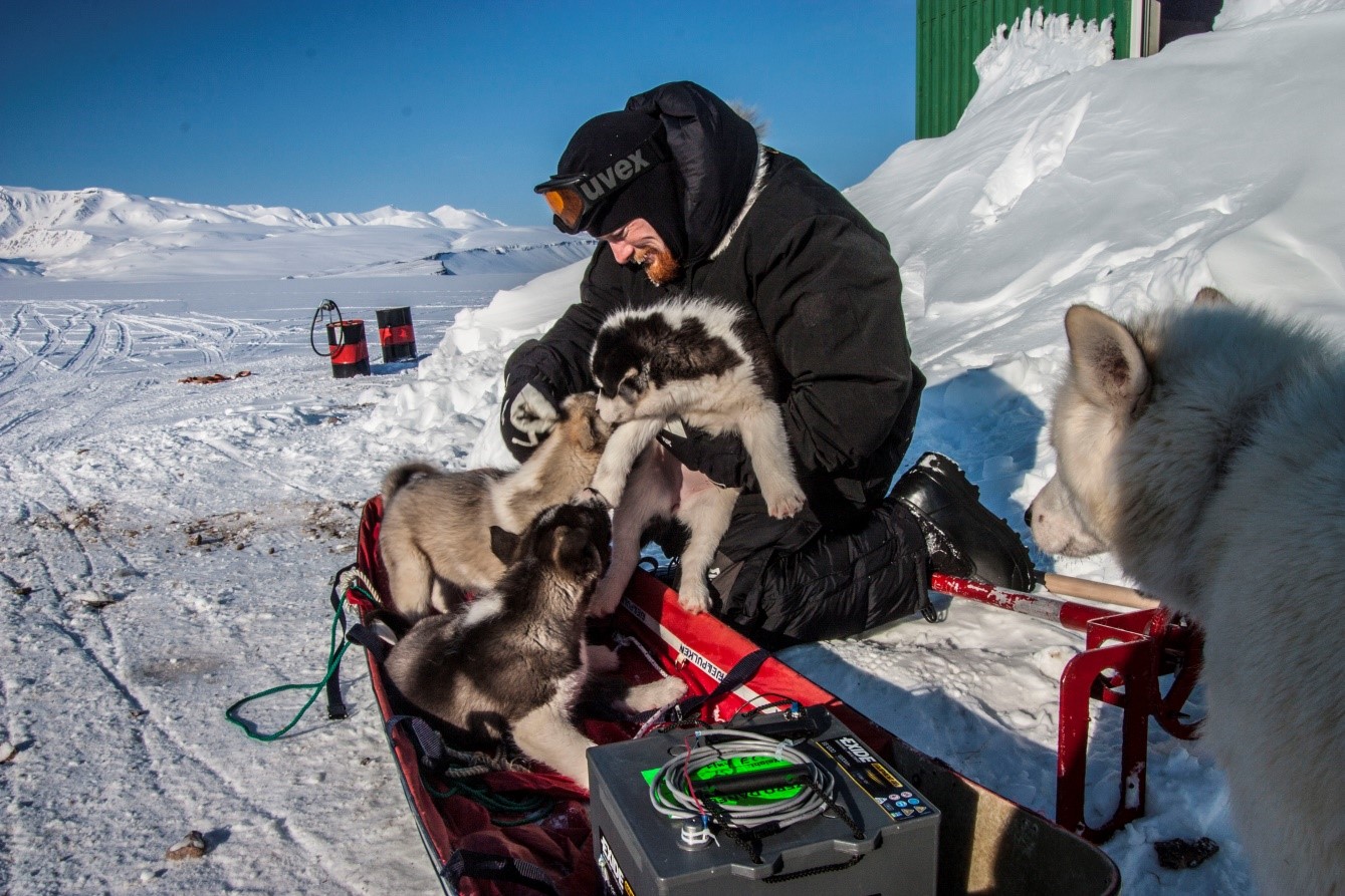
Figure 4: An unexpected challenge during fieldwork: invasion by sled dog pups. Photo: Karl Attard.

I would like to leave you with one final picture illustrating a somewhat unexpected challenge during our experiment: having to reclaim our instruments and tools from the sled dog pups (Fig. 4).

Jakob Sievers ( Arctic Research Centre / Aarhus University) has just completed his PhD at Aarhus University in Denmark as part of the DEFROST project. He is interested in the physical and biogeochemical drivers of CO2 cycling in sea-ice environments and the development of flux models and flux observation methods under these challenging circumstances. He is currently seeking funding for the purpose of continuing his research in northern Norway.