The Tibetan Plateau – area: 2.5 million km2, mean elevation: 4,700 m a.s.l., surrounded by a series of high mountain ranges that are home to some of the world’s highest peaks: Himalayas, Karakoram, Pamir, Kunlun Shan. Considering these characteristics and the unique cultural heritage of Tibet the decision was easy when I was asked if I am interested working in a project on the regional patterns of glacier change on the Tibetan Plateau. And of course, we had to do a lot of field work to collect atmospheric and glaciological data :-). Between 2009 and 2012 we could realise seven field campaigns over three to four weeks to two different glaciers.
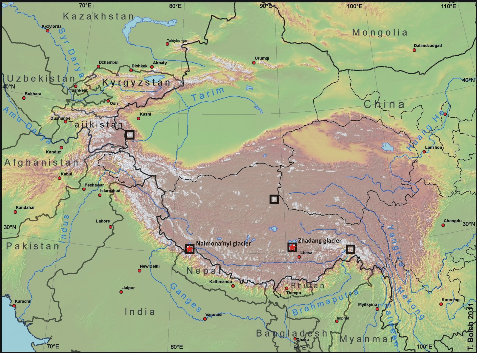
The Tibetan Plateau with location of the studied glaciers. The red stars mark the glaciers with in-situ measurements. Map by T. Bolch.
The journey always started at Lhasa airport. When leaving the plane I usually felt a little bit dizzy. Who wonders, air pressure is only 65% of that at sea level. In the following days in Lhasa every single time when walking up to the 3rd floor of our guesthouse at the Institute of Tibetan Plateau Research (ITP) I remembered that I was at 3,700 m a.s.l. By now I was glad that our schedule said that we stay in Lhasa for three nights before heading towards the snow and ice! Enough time to prepare our instruments, food and other equipment and to enjoy the tourist life… including headache and diarrhoea.
Glaciers on the Tibetan Plateau are usually terminating above 5,000 m a.s.l. and are only accessible by foot. Together with Chinese drivers and our colleagues from the ITP we left Lhasa by car, either for a one day ride to the north, to Nam Co Lake, and then another hiking day to Zhadang glacier (5,500 m a.s.l.). Or we went on a three day drive to the west, to the Kailash region, also followed by a one day ascent to Naimona’nyi glacier (5,600 m a.s.l.).
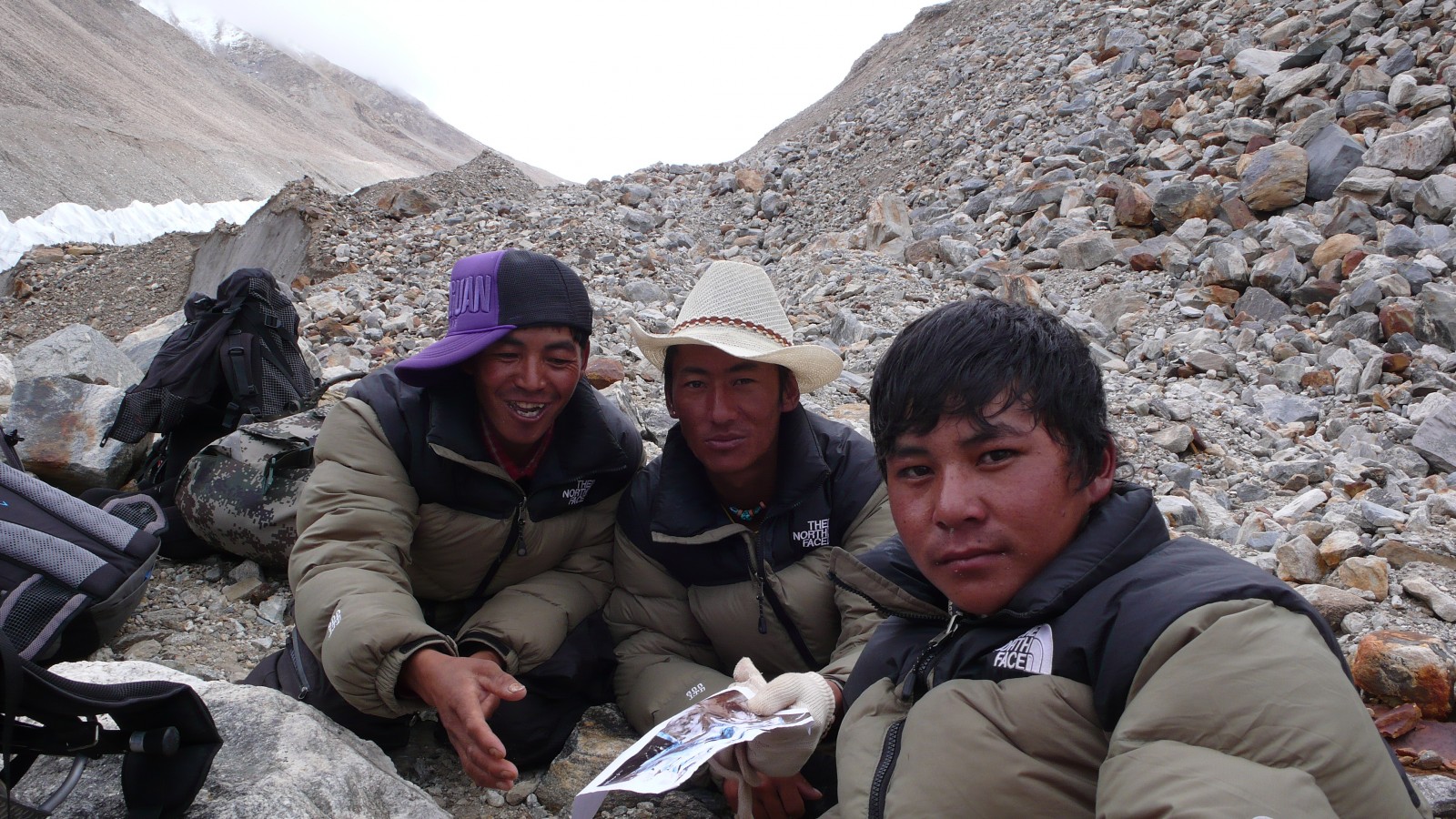
Local Tibetan people at Naimona’nyi glacier. Credit: Benjamin Schröter.
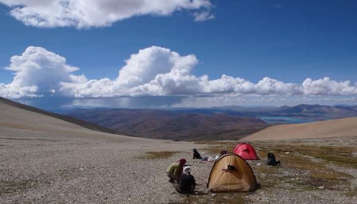
Generally, we spent two to three days in between to adapt to the altitude. With the support of local Tibetan people and yaks or horses we managed to bring all our stuff up to the glacier. I was always thankful only having to carry up myself and a small backpack :-).The torture of the ascent (at least for me) was totally forgotten when the tents were set up and we were rewarded with a great view down to the plateau (see picture at the top; camp at Naimona’nyi glacier. Credit: Benjamin Schröter).
However, we did not walk up to enjoy the landscape but to set up automatic weather stations (AWS) on or near the glacier and to conduct additional glaciological measurements. The AWS measure various atmospheric as well as surface and subsurface parameters. We also set up two time-lapse camera systems that took daily pictures of the glacier over three years. My colleagues at TU Dresden (Germany) geo-referenced and orthorectified these pictures to derive a daily snow line.
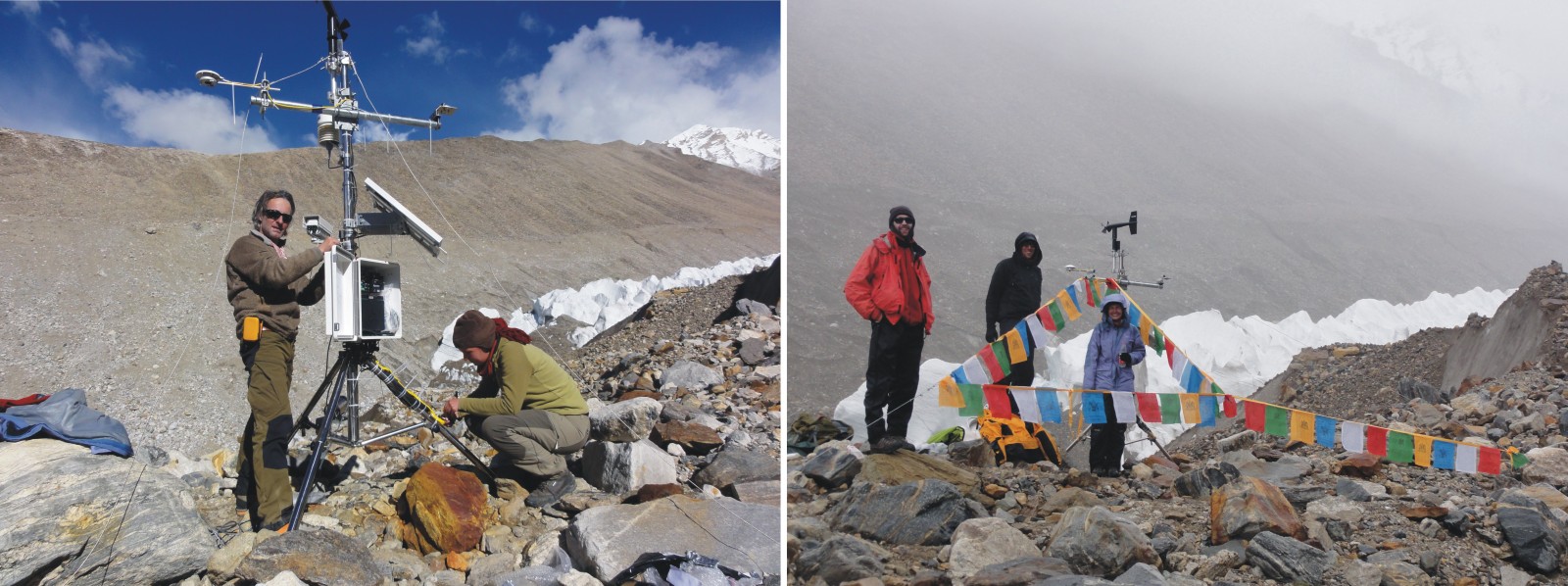
AWS at Naimona’nyi glacier in 2011. Credit: Christoph Schneider.
Usually nights up there were cold and restless and the days were quite exhausting. Air pressure drops to 50% of that at sea level. Thus, most of us were really happy when we successfully finished our measurements and repair work and walked down again after a few days to one week at the glacier side.
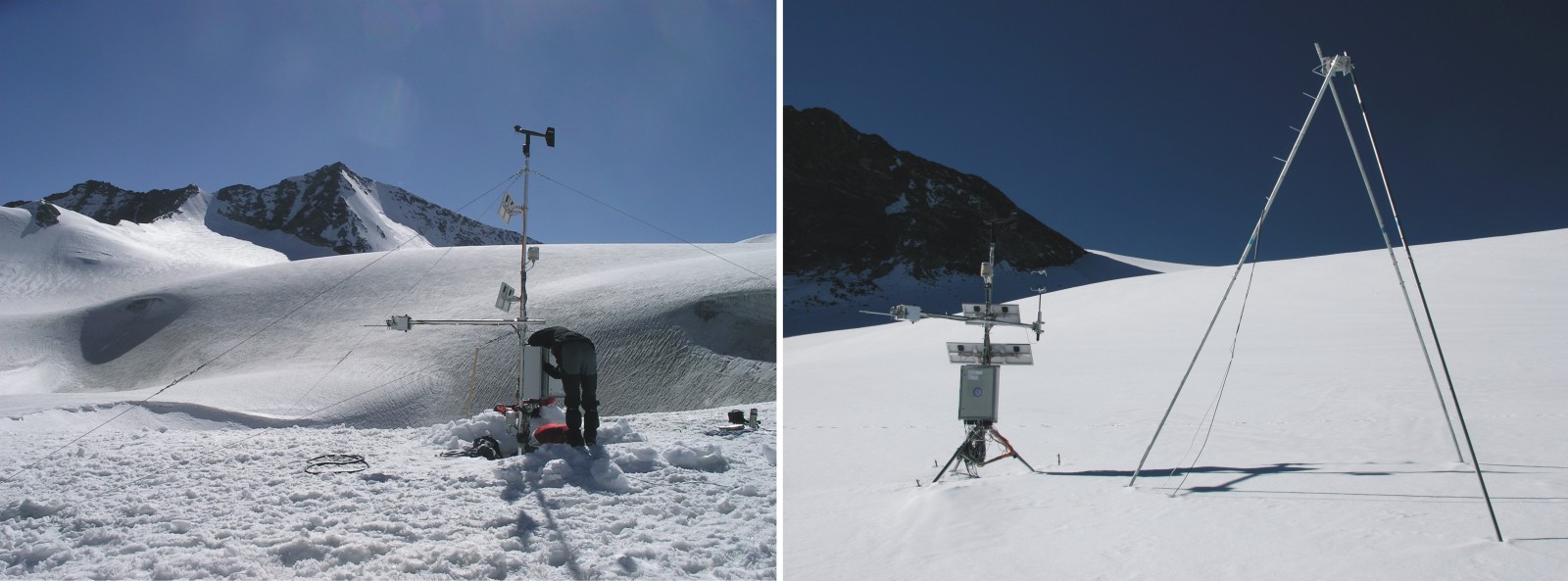
AWS at Zhadang glacier; left: 2009; right: after the ablation season in 2010. Credit: Christoph Schneider and Fabien Maussion.
When returning home in the office the real work was only just beginning. We set up a physically-based ‘COupled Snowpack and Ice surface energy and MAss balance model’ (COSIMA) that accounts for subsurface processes like melt water percolation, retention and refreezing. The collected in-situ measurements are used to calibrate, run and evaluate the model. Forced with atmospheric model data (High Asia Refined analysis; HAR) we then applied the model to five glaciers on the Tibetan Plateau (see map above). From every regional study we obtained a 10-year time series of glacier-wide surface energy and mass balance components. This data set helps us to further understand the role of the different energy and mass balance components for glacier change in the different climate regions of the Tibetan Plateau. We also hope to increase the knowledge on the various driving mechanisms for energy and mass balance on Tibetan glaciers.
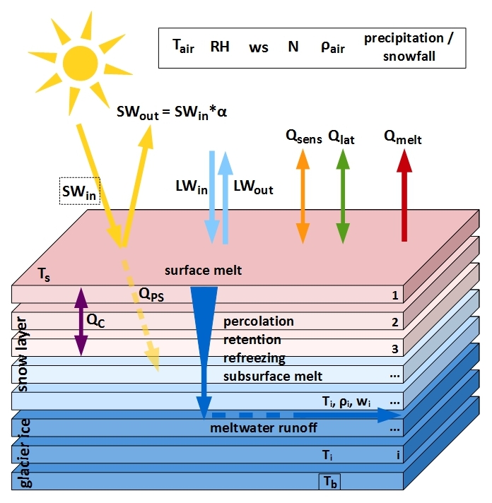
Schematic overview of COSIMA by E. Huintjes.
Illustration of the ‘COupled Snowpack and Ice surface energy and MAss balance model’ (COSIMA). Tair: air temperature; RH: relative humidity; ws: wind speed; N: cloud cover; ρair: air density; SWin: shortwave incoming radiation; SWout: shortwave outgoing radiation; α: albedo; LWin: longwave incoming radiation; LWout: longwave outgoing radiation; Qsens: turbulent sensible heat flux; Qlat: turbulent latent heat flux; Qmelt: energy flux for melting; QC: conductive heat flux; QPS: energy flux from penetrating SW radiation; Ts: surface temperature; Tb: bottom temperature; Ti: temperature of the snow/ice layer i; ρi: density of layer i; wi: liquid water content of layer i.
Follow this link to see the animated time series of the daily snow line evolution at Zhadang glacier, 2010-2012: http://www.klimageo.rwth-aachen.de/index.php?id=tibet_snowlines0&L=1
Eva Huintjes is PostDoc at RWTH Aachen University, Germany. In December 2014 she finished her PhD on ‘Energy and mass balance modelling for glaciers on the Tibetan Plateau – Extension, validation and application of a coupled snow and energy balance model’ supervised by Prof. Christoph Schneider. She is interested in understanding the different regional patterns of glacier surface energy and mass balance components and their driving mechanisms on the Tibetan Plateau and in other glaciated regions. Currently she is applying the model to glaciers in southeastern Tibet to reconstruct Little Ice Age climate conditions and to glaciers in the Tianshan (northwestern China).